Sea Surface Temperature (SST), a critical environmental element in the ocean, significantly impacts the global atmosphere-ocean energy balance and holds the potential to trigger severe weather like droughts, floods, and El Niño events. Therefore, the prediction of future SST dynamics is crucial to identifying these extreme events and mitigating the damage they caused. In this study, we introduce a time series prediction method based on the Self-Attention Mechanism-Long Short-Term Memory (SAM-LSTM) model. In addition, the historical time-series satellite data of SST anomaly (SSTA) is used instead of SST itself considering that the fluctuations of SST are very small compared to their absolute magnitudes. The Seasonal-Trend decomposition using Loess (STL) method is adopted to decompose the complex non-linear SSTA time series into trend components, seasonal components, and residual components. Then, the deseasonalized time series data at 6 locations in the Bohai Sea are used to train and valid the developed SAM-LSTM model. After that, the validated models are applied to the Yellow Sea, East China Sea, and South China Sea. The experimental results show that the combination of STL time series decomposition and SAM-LSTM can achieve high-precision prediction of daily SSTA than LSTM. This suggests that the methodology used in this paper has a good application for short-term daily SST prediction.
This is an Open Access article, distributed under the terms of the Creative Commons Attribution 4.0 International License (http://creativecommons.org/licenses/by/4.0/), which permits unrestricted use, distribution and reproduction in any medium or format, provided the original work is properly cited.
Long Short-Term Memory (LSTM), Self-Attention Mechanism (SAM), Sea Surface Temperature (SST), Seasonal-Trend Decomposition Using Loess (STL)
1. Introduction
Sea Surface Temperature (SST), a critical environmental element in the ocean, has significant impacts on the transfer of energy, momentum, and moisture between the ocean and the atmosphere. Changes in SST can influence the global atmosphere-ocean energy cycle and potentially result in calamities such as droughts, floods, and El Niño events
[1
-3]. Therefore, predicting SST has become a focal point of current research. Accurately predicting SST has significant scientific and practical importance. However, due to the influence of multiple factors, the accuracy of SST prediction in coastal areas is frequently low.
Methods for predicting SST include numerical models and data-driven models. In numerical model studies, researchers establish complex thermodynamic and physical equations based on physical and chemical indicators in the ocean to predict SST
[4]
Noori, R., Abbasi, M. R., Adamowski, J. F., et al. A simple mathematical model to predict sea surface temperature over the northwest Indian Ocean. Estuarine, Coastal and Shelf Science, 2017, 197: 236-243.
5]. However, numerical methods are based on physical conditions and processes, causing computational complexity and laborious processes
[6]
Stockdale, T. N., Balmaseda, M. A., Vidard, A. Tropical Atlantic SST Prediction with Coupled Ocean–Atmosphere GCMs. Journal of Climate, 2006, 19(23): 6047-6061.
Sadeghi, H., Kniesburges, S., Kaltenbacher, M., et al. Computational Models of Laryngeal Aerodynamics: Potentials and Numerical Costs. Journal of Voice, 2019, 33(4): 385-400.
. Additionally, they are typically used for coarse resolution large area predictions rather than specific fine resolution site predictions
[9]
Krishnamurti, T. N., Chakraborty, A., Krishnamurti, R., et al. Seasonal Prediction of Sea Surface Temperature Anomalies Using a Suite of 13 Coupled Atmosphere–Ocean Models. Journal of Climate, 2006, 19(23): 6069-6088.
. The data-driven methods can be divided into two categories: traditional statistical methods and emerging machine learning methods. Statistical methods include Markov models, canonical correlation analysis, and empirical orthogonal functions
[10]
Kug, J. S., Kang, I. S., Lee, J. Y., et al. A statistical approach to Indian Ocean sea surface temperature prediction using a dynamical ENSO prediction. Geophysical Research Letters, 2004, 31(9): L09212.
Hannachi, A., Jolliffe, I. T., Stephenson, D. B. Empirical orthogonal functions and related techniques in atmospheric science: A review. International Journal of Climatology, 2007, 27(9): 1119-1152.
Asahara, A., Maruyama, K., Sato, A., et al. Pedestrian-movement prediction based on mixed Markov-chain model. In Proceedings of the 19th ACM SIGSPATIAL International Conference on Advances in Geographic Information Systems. New York, USA, 2011; pp: 25-33.
. However, these methods can only model linear relationships and lack the ability to model complex nonlinear processes
[13]
Lee, J. W., Hodgkiss, I. J., Wong, K. M., et al. Real time observations of coastal algal blooms by an early warning system. Estuarine, Coastal and Shelf Science, 2005, 65(1): 172-190.
. Conversely, machine learning methods based on data, can model non-stationary and nonlinear patterns in SST time series and have been proven to produce satisfactory predictive results. Various neural network models have been used for predicting SST under different variations
[15]
Patil, K., Deo, M. C., Ghosh, S., et al. Predicting Sea Surface Temperatures in the North Indian Ocean with Nonlinear Autoregressive Neural Networks. International Journal of Oceanography, 2013, 2013: 1-11.
Aparna, S. G., D’Souza, S., Arjun, N. B. Prediction of daily sea surface temperature using artificial neural networks. International Journal of Remote Sensing, 2018, 39(12): 4214-4231.
. For instance, Zhang et al. proposed an LSTM-based network to model the temporal relationships of SST to predict future values, making the recurrent neural networks to address the SST prediction problem first time
[18]
Zhang, Q., Wang, H., Dong, J., et al. Prediction of Sea Surface Temperature Using Long Short-Term Memory. IEEE Geoscience and Remote Sensing Letters, 2017, 14(10): 1745-1749.
Fan, S., Xiao, N., Dong, S. A novel model to predict significant wave height based on long short-term memory network. Ocean Engineering, 2020, 205: 107298.
Song, T., Jiang, J., Li, W., et al. A Deep Learning Method with Merged LSTM Neural Networks for SSHA Prediction. IEEE Journal of Selected Topics in Applied Earth Observations and Remote Sensing, 2020, 13: 2853-2860.
. Despite LSTM delivering commendable results in time series prediction tasks, its high complexity gives rise to issues such as overfitting. Therefore, to enhance the predictive accuracy of SST remains a critical issue.
To reduce the error of the LSTM model's prediction results and further improve the prediction results, it may be considered to combine it with other prediction techniques in some way. In this paper, we attempt to combine it with Self-Attention Mechanism (SAM). This approach is based on research into human vision and has been introduced into the fields of computer vision, natural language processing and others to optimize existing models
[22]
Han, K. J., Prieto, R., Ma, T. State-of-the-Art Speech Recognition Using Multi-Stream Self-Attention with Dilated 1D Convolutions. In 2019 IEEE Automatic Speech Recognition and Understanding Workshop (ASRU). Singapore, 2019; pp: 54-61.
Kim, J., El-Khamy, M., Lee, J. T-GSA: Transformer with Gaussian-Weighted Self-Attention for Speech Enhancement. In 2020 IEEE International Conference on Acoustics, Speech and Signal Processing (ICASSP). Barcelona, Spanish, 2020; pp: 6649-6653.
Zhao, H., Jia, J., Koltun, V. Exploring Self-Attention for Image Recognition. In 2020 IEEE Conference on Computer Vision and Pattern Recognition (CVPR). Seattle, USA, 2020; pp: 10073-10082.
. In this way, the model can effectively capture global dependencies and extract information from previously aggregated features, enhancing its ability to identify relevant information.
Therefore, the research objectives of this paper include the following: 1) develop LSTM deep neural network models that can predict short and mid-term SST with high accuracy; 2) improve the LSTM model based on the SAM to achieve more accurate predictions; and 3) conduct experiments at selected sites in the China Sea utilizing 41 years of satellite time-series data to examine the applicability, effectiveness and advantages of the proposed combined SAM-LSTM model in predicting the short and mid-term daily SST.
The remainder of the paper is organized as follows: Section 2 describes the study area and the time-series SST data from the satellite inversion used in this study, and the prediction methodology. Section 3 gives the experimental results. Section 4 and 5 present the discussions and conclusions of this study.
2. Materials and Methods
2.1. Study Area
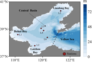
The study area is the Bohai Sea in China. The Bohai Sea consists of Bohai Bay, Laizhou Bay, Liaodong Bay, the Yellow River Estuary, and the central sea area. And the Bohai Sea acts as a migration area for various economic fish species, possessing rich biological resources. Therefore, predicting the dynamics of sea temperature in this area is crucial for research. In addition, research has shown that the coastal sea of China (mainly including the nearshore and offshore areas of the Bohai Sea, Yellow Sea, East China Sea, and South China Sea) is a marginal sea of the western North Pacific. Notably, against the background of global warming, this region has become a key area for exploring typical climate and environmental changes and causes in China, particularly the eastern mainland and coastal areas. Therefore, achieving accurate prediction of SST in the China Seas is significant for the protection of national seas, ecological protection, and the development of agricultural and trade economies.
In this study, we select 6 representative sites in the Bohai Sea as the study locations. These 6 sites differ in their distance from the shoreline, as shown in Figure 1. The 6 sites are denoted as L1-L6, where L1-L3 are located in the nearshore area, and L4-L6 are located in the offshore area.
Figure 1. The study area is located in the Bohai Sea.
2.2. Data Sources
Long time series satellite data is an excellent option for predicting marine environment time series. Therefore, the data used in this paper is the National Oceanic and Atmospheric Administration (NOAA) 1/4° daily Optimum Interpolation Sea Surface Temperature (daily OISST, version 2), with the time range of September 1981 to December 2023. Given the small deviations in SST in comparison to its absolute magnitude, the preference is for utilizing Sea Surface Temperature Anomaly (SSTA) for modeling. The SSTA is a variable of OISST-V2-AVHRR data, which is calculated relative to 1971-2000 climatology (PSD).
The basic statistical information of SSTA at 6 observation sites (L1-L6) is presented in Table 1 for SSTA time series prediction analysis. This allows us to observe the size and fluctuation range of the SSTA data.
Table 1. Statistics of the SSTA time series at L1 to L6 from 1982/01/01 to 2023/12/31.
Sites
Mean (°C)
Std (°C)
Min (°C)
Max (°C)
Median (°C)
L1
0.61
1.89
-4.82
8.59
0.31
L2
-0.52
1.69
-4.42
6.89
0.41
L3
-0.16
1.43
-5.05
5.13
-0.27
L4
0.15
1.15
-4.16
4.65
0.15
L5
0.44
1.16
-3.82
4.94
0.43
L6
0.01
1.18
-4.70
4.33
0.02
2.3. Method
2.3.1. LSTM Deep Neural Networks
The LSTM model has the capability to capture long-term sequential information in time series data. Therefore, this paper utilizes the LSTM model for making predictions on time series data. LSTM is an expanded form of the Recurrent Neural Networks (RNN) structure, where each LSTM unit contains a memory cell and three gates: forget gate, input gate, and output gate
[25]
Hochreiter, S., Schmidhuber, J. Long Short-Term Memory. Neural Computation, 1997, 9(8): 1735-1780.
. These gates regulate the flow of information associated with the memory cell state. The forget gate determines the amount of memory cell state passed through the current LSTM unit, the input gate uses current input and previous hidden state information to update the memory cell state, and the output gate controls the selective output of the current memory cell state. These options enable LSTM to understand temporal relationships in lengthy sequences. The formula for information state transmission in a single LSTM unit is as follows:
(1)
(2)
(3)
(4)
(5)
Where is the Hadamard product, is the sigmoid activation function, tanh is the activation function, stands for the input gate, represents the forget gate, represents the output cell, represents the current cell state, represents the cell state at the previous moment, represents the final output, represents the weight coefficient of the given gate, and is the corresponding bias coefficient of the given gate.
2.3.2. Self-Attention Mechanisms
Self-Attention Mechanism is an attention mechanism that has been studied in natural language processing and computer vision. The mechanism can be formulated as equation (6), where is Query, is Key, and is Value. These three terms are matrices, all of which are of size , and are is the dimension of Key.
(6)
The mechanism reduces the effect of variance on the network gradient update by transposing by and dividing each element of the similarity matrix by . Then, the results are normalized by applying a softmax function to obtain the corresponding weight coefficient matrix. Finally, the resulting matrix is multiplied by . In this way, the model can effectively capture global dependencies and obtain information from past aggregated features, enhancing the ability to recognize complex moving objects.
2.3.3. SAM-LSTM Combined Modeling
This paper develops a deep neural network model using SAM and LSTM for predicting specific site SSTA, as illustrated in Figure 2. The model takes SSTA time series as input and employs the rolling prediction method. For each LSTM model training, historical observed values are utilized to establish a pattern between the SSTA at time and its previous values at time , ,…and (referred to as time window). Then, future predictions are made based on the identified pattern and sliding the time window, allowing for predictions days ahead. Therefore, the prediction approach in this paper involves inputting the SSTA sequence in the form of a time window into the LSTM layer to extract time features. Then input the sequence processed by the SAM layer for enhanced information extraction, and obtain the final prediction result through the Dense layer. The latest prediction is used to update the input SSTA sequence for predicting daily SSTA.
2.4. Model Evaluation Indicators
The performance of the SSTA prediction method is measured using three metrics: mean absolute error (MAE), root mean square error (RMSE), and coefficient of determination (R2). These are defined as follows:
(7)
(8)
(9)
where and represent the actual and predicted values, respectively, represents the average actual value, represents the sample size, and represents the value.
3. Results
3.1. Data Pre-processing
Before feeding the historical SSTA observations into the SAM-LSTM model for training, the SSTA time series at each selected location are first deseasonalized and normalized. Deseasonalization is useful for exploring trends, cycles, and any remaining irregular components of the time series and has been shown to contribute to more accurate predictions than using original data
[26]
Nelson, M., Hill, T., Remus, W., et al. Time series predicting using neural networks: should the data be deseasonalized first? Journal of Predicting, 1999, 18(5): 359-367.
. Therefore, we have first predicted the deseasonalized SSTA data. Then, seasonality is added to obtain the final prediction. In addition, the deseasonalized SSTA time series for each site are normalized to make the data more centralized, which facilitates the functioning of the model.
Figure 2. The architecture of the SAM-LSTM deep neural network model for SSTA prediction.
Table 2. The Yellow Sea, East China Sea and South China Sea Station Location.
The Yellow Sea
The East China Sea
The South China Sea
Nearshore
L7 (121.00°E, 35.66°N)
L9 (123.20°E, 28.63°N)
L11 (114.60°E, 21.26°N)
Offshore
L8 (123.40°E, 35.27°N)
L10 (126.35°E, 29.46°N)
L12 (116.06°E, 18.66°N)
3.2. Trend Decomposition
Seasonal-Trend decomposition using Loess (STL) is a reliable method for decomposing time series data into seasonal, trend, and residual components. Loess is an algorithm for dealing with nonlinear correlation. STL is ideal for time series decomposition because it can address any type of seasonality. When performing time series decomposition, the time series has three main components: the trend, seasonal and residual components. Two commonly used time series decompositions are additive and multiplicative decompositions, whose expressions are shown in (10) and (11).
(10)
(11)
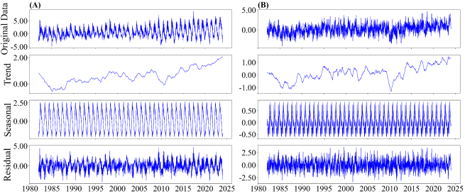
The additive decomposition method is employed in this study to decompose the SSTA time series, as the magnitude of seasonal fluctuations and the change in trend do not vary with the time series. Since the decomposition plots of the three points on the nearshore are similar, and the same is true for the offshore, this paper only shows the decomposition plots of the L1 position on the nearshore and the L4 position on the offshore, and the results of the decompositions are shown in Figure 3.
The original SSTA time series exhibits strong instability. The trend component after the STL decomposition greatly restores the changing trend of the original SSTA time series. The SSTA at 6 sites shows an increasing trend from 1982 to 2023, with a more significant rise in the nearshore area. The seasonal component shows very consistent frequency of change, mainly extracting the seasonal variation attributes of the original time series. The seasonal changes at 3 nearshore sites are very similar, as are the seasonal changes at three offshore sites. The residual component lacks a distinct changing pattern compared to the trend and seasonal components.
3.3. Experimental Setup
For the SSTA prediction experiments at each location, we set the time window of the input SSTA sequence to 40. The datasets are prepared for LSTM and SAM-LSTM models (LSTM is used for comparison). The SSTA data from 1982/01/01 to 2010/12/31 is used as the training set, while the SSTA data from 2011/01/01 to 2017/12/31 is used for validation, and the remaining samples are used for the final model test to evaluate the model's performance. The SSTA prediction is conducted at 6 sites in the Bohai Sea, as described in Section 2.1.
Figure 3. STL decomposition of L1 and L4 locations in the Bohai Sea: original data, trend, seasonal and residual components in sequence.
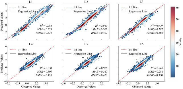
3.4. SSTA Predictive Model Validation
The use of conventional scatter regression plots is inadequate for effectively depicting the prediction effect due to large data. Therefore, a density scatter plot is employed to display the prediction. Figures 4 and 5 show the results of the density scatter plots for the validation and test sets at the 6 locations in the Bohai Sea. The results of the density scatterplot indicate that the SAM-LSTM model developed in this study shows outstanding performance on both the validation and test sets. Among the three prediction models near the shore, the L1 location exhibits superior performance on both the validation and test sets, whereas the L3 location shows slightly inferior prediction performance. On the offshore, the L6 location demonstrates significantly better performance on both the validation and test sets, while the L4 location shows relatively poor performance. The R2 of the nearshore locations are all higher than 0.95, the MAE is lower than 0.26, and the RMSE is concentrated in 0.368 to 0.464, with ideal model performance. The R2 of the offshore locations are all higher than 0.89, the MAE is lower than 0.28, and the RMSE is concentrated in 0.39 to 0.494, and the prediction performance of the offshore locations is relatively lower than the nearshore locations. This may be attributed to the relatively stable trend components of the nearshore locations, showing an almost yearly increasing trend. In contrast, the trend components of the offshore locations are unstable and the increasing trend of SSTA is relatively less pronounced compared to the nearshore. As a result, the model is more effective in capturing the SSTA change trend nearshore, leading to better prediction performance compared to offshore. This observation should be taken into account in future research by incorporating dynamic conditions and other factors influencing offshore SST.
Figure 5. The Density Scatterplot of the testing set for SSTA prediction.
3.5. Application of SAM-LSTM SSTA Prediction Modeling
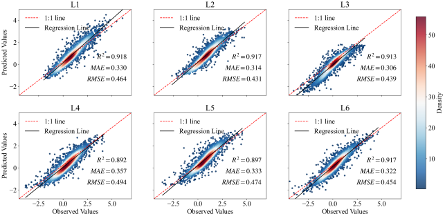
The results of the previous section show that model 1 (L1 location) and model 6 (L6 location) are the best predictive models for the nearshore and offshore, respectively. To demonstrate the generalizability of the models, a location site is selected in the Yellow Sea, East China Sea and South China Sea areas nearshore and offshore, respectively, and the specific location information is shown in Table 2. The input data collected from three specified ocean regions during the period from 2018/01/01 to 2018/02/09 is utilized as the input for predicting the SSTA values for the future two months. L7, L9, L11 are predicted by model 1 (L1 location), and L8, L10, L12 are predicted by model 6 (L6 location).
Figure 6 illustrates the outstanding performance of the SAM-LSTM model, with R2 exceeding 0.9, MAE below 0.3, and RMSE mainly concentrated between 0.3 and 0.5. However, it performs poorly in predicting certain high and low values for both the nearshore and offshore. In the prediction of SSTA at nearshore and offshore sites in three sea areas, we could observe significant high and low SSTA values. The high values can reach 6°C, and the low values can reach -4°C. Prediction errors are primarily concentrated at the extremes of high and low values. Analysis of the SSTA line graphs for the 3 sea areas shows that when there is a large change in SSTA, the predictive capacity of the model significantly reduces. This is attributed to the substantial data change, which hinders the model's ability to accurately capture the trend for the next moment, resulting in error accumulation.
Figure 6. (A) The nearshore L7, L9, and L11 locations are partially sampled in the L1 prediction model for 1 day ahead; (B) The nearshore L8, L10, and L12 locations are partially sampled in the L6 prediction model for 1 day ahead.
4. Discussion
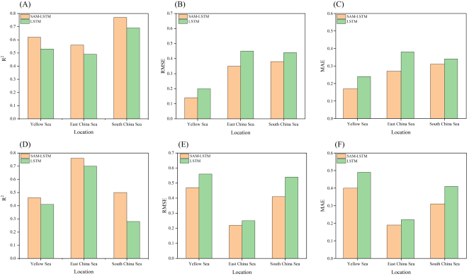
All the above results show that the SAM-LSTM model has satisfactory prediction performance. To further prove the prediction performance of SAM-LSTM, the prediction results for 10 days are used to fully demonstrate that the SAM-LSTM model proposed in this paper is superior to the traditional LSTM. Except without the self-attention mechanism, all the other model parameters of the LSTM are the same as the settings of the SAM-LSTM model. The specific operation is to use the prediction models at L1-L6 positions to predict the SSTA for the next 10 days for the nearshore and offshore of the Yellow Sea, the East China Sea and the South China Sea, respectively. And obtaining an average nearshore model and an average offshore model for each sea area, and then conducting relevant analysis, as shown in Figure 7.
Observing the R2 histograms of nearshore and offshore, it can be clearly seen that the R2 of nearshore and offshore of the SAM-LSTM model is higher than LSTM in the prediction of the next 10 days. Among them, the South China Sea has the highest R2 in the nearshore prediction, and the East China Sea has the highest R2 in the offshore prediction. In addition, the R2 of the nearshore is higher than that of the offshore, which is consistent with the prediction of the Bohai Sea. The results of the RMSE histograms show that the RMSE of the Yellow Sea is the lowest in the nearshore, and the RMSE of the East Sea is the lowest in the offshore. In addition, the RMSE of the SAM-LSTM model is lower than the LSTM model in all the sea areas in both nearshore and offshore. From the MAE histograms, it can be observed that the MAE of the Yellow Sea is the lowest in the nearshore, the East Sea is the lowest in the offshore, and the MAE of the SAM-LSTM model is lower than the LSTM model.
In summary, the prediction performance of the SAM-LSTM model constructed in this paper outperforms the traditional LSTM deep neural network model in the short and mid-term prediction experiments for the next 10 days, and it can be applied to the Yellow Sea, the East China Sea and the South China Sea for the SSTA prediction. However, only SSTA data are considered in this paper, and the SST is affected by various factors such as solar radiation and atmospheric motion. Therefore, a multivariate prediction model should be considered in the future to further improve the model prediction performance, so that the sudden and frequent occurrence of ecological disasters (such as red tide) can be effectively prevented.
Figure 7. Comparison of the prediction performance of SAM-LSTM and LSTM (10 days). (A)-(C) are the R2, RMSE, and MAE in the nearshore, respectively; (D)-(F) are the R2, RMSE, and MAE in the offshore.
5. Conclusions
In order to achieve precise short mid-term daily SST prediction, this paper introduces a time series predicting method based on the SAM-LSTM model. It utilizes 41 years of daily SST time series data obtained from the AVHRR satellite sensor at 6 locations in the Bohai Sea for training and testing. In this approach, considering the small fluctuation of sea temperature relative to its absolute magnitude. The STL time series decomposition method is employed to decompose the complex non-linear time series into trend components, seasonal components, and residual components. Then, the SAM-LSTM models of 6 sites are constructed to predict the deseasonalized future SSTA, effectively reducing the model fitting difficulty and decreasing prediction errors. The validated and tested models are applied to the Yellow Sea, East China Sea, and South China Sea, and SAM-LSTM is compared with LSTM. The conclusions are as follows:
(1) The combination of STL time series decomposition and the SAM-LSTM model can achieve high-precision prediction of daily SSTA, with better predictive performance at nearshore locations than offshore locations.
(2) The validated and tested models exhibit excellent predictive performance in the Yellow Sea, East China Sea, and South China Sea, with R2 values all above 0.9, MAE below 0.3, and RMSE mainly ranging from 0.2 to 0.5.
(3) Comparing SAM-LSTM and LSTM using different statistics such as R2, RMSE, and MAE, it is evident that LSTM with the addition of SAM can achieve more accurate prediction.
Abbreviations
LSTM: Long Short-Term Memory
SAM: Self-Attention Mechanism
SST: Sea Surface Temperature
SSTA: Sea Surface Temperature Anomaly
STL: Seasonal-Trend Decomposition Using Loess
Conflicts of Interest
The authors declare no conflicts of interest.
References
[1]
Bouali, M., Sato, O. T., Polito, P. S. Temporal trends in sea surface temperature gradients in the South Atlantic Ocean. Remote Sensing of Environment, 2017, 194: 100-114.
Yao, S. L., Luo, J. J., Huang, G., et al. Distinct global warming rates tied to multiple ocean surface temperature changes. Nature Climate Change, 2017, 7(7): 486-491.
Noori, R., Abbasi, M. R., Adamowski, J. F., et al. A simple mathematical model to predict sea surface temperature over the northwest Indian Ocean. Estuarine, Coastal and Shelf Science, 2017, 197: 236-243.
Sarkar, P. P., Janardhan, P., Roy, P. Prediction of sea surface temperatures using deep learning neural networks. SN Applied Sciences, 2020, 2(8): 1458.
Stockdale, T. N., Balmaseda, M. A., Vidard, A. Tropical Atlantic SST Prediction with Coupled Ocean–Atmosphere GCMs. Journal of Climate, 2006, 19(23): 6047-6061.
Sadeghi, H., Kniesburges, S., Kaltenbacher, M., et al. Computational Models of Laryngeal Aerodynamics: Potentials and Numerical Costs. Journal of Voice, 2019, 33(4): 385-400.
Krishnamurti, T. N., Chakraborty, A., Krishnamurti, R., et al. Seasonal Prediction of Sea Surface Temperature Anomalies Using a Suite of 13 Coupled Atmosphere–Ocean Models. Journal of Climate, 2006, 19(23): 6069-6088.
Kug, J. S., Kang, I. S., Lee, J. Y., et al. A statistical approach to Indian Ocean sea surface temperature prediction using a dynamical ENSO prediction. Geophysical Research Letters, 2004, 31(9): L09212.
Hannachi, A., Jolliffe, I. T., Stephenson, D. B. Empirical orthogonal functions and related techniques in atmospheric science: A review. International Journal of Climatology, 2007, 27(9): 1119-1152.
Asahara, A., Maruyama, K., Sato, A., et al. Pedestrian-movement prediction based on mixed Markov-chain model. In Proceedings of the 19th ACM SIGSPATIAL International Conference on Advances in Geographic Information Systems. New York, USA, 2011; pp: 25-33.
Lee, J. W., Hodgkiss, I. J., Wong, K. M., et al. Real time observations of coastal algal blooms by an early warning system. Estuarine, Coastal and Shelf Science, 2005, 65(1): 172-190.
Patil, K., Deo, M. C., Ghosh, S., et al. Predicting Sea Surface Temperatures in the North Indian Ocean with Nonlinear Autoregressive Neural Networks. International Journal of Oceanography, 2013, 2013: 1-11.
Aparna, S. G., D’Souza, S., Arjun, N. B. Prediction of daily sea surface temperature using artificial neural networks. International Journal of Remote Sensing, 2018, 39(12): 4214-4231.
Zhang, Q., Wang, H., Dong, J., et al. Prediction of Sea Surface Temperature Using Long Short-Term Memory. IEEE Geoscience and Remote Sensing Letters, 2017, 14(10): 1745-1749.
Fan, S., Xiao, N., Dong, S. A novel model to predict significant wave height based on long short-term memory network. Ocean Engineering, 2020, 205: 107298.
Song, T., Jiang, J., Li, W., et al. A Deep Learning Method with Merged LSTM Neural Networks for SSHA Prediction. IEEE Journal of Selected Topics in Applied Earth Observations and Remote Sensing, 2020, 13: 2853-2860.
Han, K. J., Prieto, R., Ma, T. State-of-the-Art Speech Recognition Using Multi-Stream Self-Attention with Dilated 1D Convolutions. In 2019 IEEE Automatic Speech Recognition and Understanding Workshop (ASRU). Singapore, 2019; pp: 54-61.
Kim, J., El-Khamy, M., Lee, J. T-GSA: Transformer with Gaussian-Weighted Self-Attention for Speech Enhancement. In 2020 IEEE International Conference on Acoustics, Speech and Signal Processing (ICASSP). Barcelona, Spanish, 2020; pp: 6649-6653.
Zhao, H., Jia, J., Koltun, V. Exploring Self-Attention for Image Recognition. In 2020 IEEE Conference on Computer Vision and Pattern Recognition (CVPR). Seattle, USA, 2020; pp: 10073-10082.
Nelson, M., Hill, T., Remus, W., et al. Time series predicting using neural networks: should the data be deseasonalized first? Journal of Predicting, 1999, 18(5): 359-367.
Song, J., Zhang, X., Jiang, W. (2024). Sea Surface Temperature Prediction in China Sea Based on SAM-LSTM Approach. American Journal of Environmental Science and Engineering, 8(2), 14-22. https://doi.org/10.11648/j.ajese.20240802.11
Song, J.; Zhang, X.; Jiang, W. Sea Surface Temperature Prediction in China Sea Based on SAM-LSTM Approach. Am. J. Environ. Sci. Eng.2024, 8(2), 14-22. doi: 10.11648/j.ajese.20240802.11
Song J, Zhang X, Jiang W. Sea Surface Temperature Prediction in China Sea Based on SAM-LSTM Approach. Am J Environ Sci Eng. 2024;8(2):14-22. doi: 10.11648/j.ajese.20240802.11
@article{10.11648/j.ajese.20240802.11,
  author = {Jiali Song and Xueqing Zhang and Wensheng Jiang},
  title = {Sea Surface Temperature Prediction in China Sea Based on SAM-LSTM Approach
},
  journal = {American Journal of Environmental Science and Engineering},
  volume = {8},
  number = {2},
  pages = {14-22},
  doi = {10.11648/j.ajese.20240802.11},
  url = {https://doi.org/10.11648/j.ajese.20240802.11},
  eprint = {https://article.sciencepublishinggroup.com/pdf/10.11648.j.ajese.20240802.11},
  abstract = {Sea Surface Temperature (SST), a critical environmental element in the ocean, significantly impacts the global atmosphere-ocean energy balance and holds the potential to trigger severe weather like droughts, floods, and El Niño events. Therefore, the prediction of future SST dynamics is crucial to identifying these extreme events and mitigating the damage they caused. In this study, we introduce a time series prediction method based on the Self-Attention Mechanism-Long Short-Term Memory (SAM-LSTM) model. In addition, the historical time-series satellite data of SST anomaly (SSTA) is used instead of SST itself considering that the fluctuations of SST are very small compared to their absolute magnitudes. The Seasonal-Trend decomposition using Loess (STL) method is adopted to decompose the complex non-linear SSTA time series into trend components, seasonal components, and residual components. Then, the deseasonalized time series data at 6 locations in the Bohai Sea are used to train and valid the developed SAM-LSTM model. After that, the validated models are applied to the Yellow Sea, East China Sea, and South China Sea. The experimental results show that the combination of STL time series decomposition and SAM-LSTM can achieve high-precision prediction of daily SSTA than LSTM. This suggests that the methodology used in this paper has a good application for short-term daily SST prediction.
},
 year = {2024}
}
TY  - JOUR
T1  - Sea Surface Temperature Prediction in China Sea Based on SAM-LSTM Approach

AU  - Jiali Song
AU  - Xueqing Zhang
AU  - Wensheng Jiang
Y1  - 2024/04/28
PY  - 2024
N1  - https://doi.org/10.11648/j.ajese.20240802.11
DO  - 10.11648/j.ajese.20240802.11
T2  - American Journal of Environmental Science and Engineering
JF  - American Journal of Environmental Science and Engineering
JO  - American Journal of Environmental Science and Engineering
SP  - 14
EP  - 22
PB  - Science Publishing Group
SN  - 2578-7993
UR  - https://doi.org/10.11648/j.ajese.20240802.11
AB  - Sea Surface Temperature (SST), a critical environmental element in the ocean, significantly impacts the global atmosphere-ocean energy balance and holds the potential to trigger severe weather like droughts, floods, and El Niño events. Therefore, the prediction of future SST dynamics is crucial to identifying these extreme events and mitigating the damage they caused. In this study, we introduce a time series prediction method based on the Self-Attention Mechanism-Long Short-Term Memory (SAM-LSTM) model. In addition, the historical time-series satellite data of SST anomaly (SSTA) is used instead of SST itself considering that the fluctuations of SST are very small compared to their absolute magnitudes. The Seasonal-Trend decomposition using Loess (STL) method is adopted to decompose the complex non-linear SSTA time series into trend components, seasonal components, and residual components. Then, the deseasonalized time series data at 6 locations in the Bohai Sea are used to train and valid the developed SAM-LSTM model. After that, the validated models are applied to the Yellow Sea, East China Sea, and South China Sea. The experimental results show that the combination of STL time series decomposition and SAM-LSTM can achieve high-precision prediction of daily SSTA than LSTM. This suggests that the methodology used in this paper has a good application for short-term daily SST prediction.

VL  - 8
IS  - 2
ER  -
College of Environmental Science and Engineering, Ocean University of China, Qingdao, China; Key Laboratory of Marine Environment and Ecology, Ministry of Education of China, Ocean University of China, Qingdao, China; Sanya Oceanographic Institution (Ocean University of China), Yazhou Bay Science and Technology City, Sanya, China
College of Environmental Science and Engineering, Ocean University of China, Qingdao, China; Key Laboratory of Marine Environment and Ecology, Ministry of Education of China, Ocean University of China, Qingdao, China
College of Environmental Science and Engineering, Ocean University of China, Qingdao, China; Key Laboratory of Marine Environment and Ecology, Ministry of Education of China, Ocean University of China, Qingdao, China
Song, J., Zhang, X., Jiang, W. (2024). Sea Surface Temperature Prediction in China Sea Based on SAM-LSTM Approach. American Journal of Environmental Science and Engineering, 8(2), 14-22. https://doi.org/10.11648/j.ajese.20240802.11
Song, J.; Zhang, X.; Jiang, W. Sea Surface Temperature Prediction in China Sea Based on SAM-LSTM Approach. Am. J. Environ. Sci. Eng.2024, 8(2), 14-22. doi: 10.11648/j.ajese.20240802.11
Song J, Zhang X, Jiang W. Sea Surface Temperature Prediction in China Sea Based on SAM-LSTM Approach. Am J Environ Sci Eng. 2024;8(2):14-22. doi: 10.11648/j.ajese.20240802.11
@article{10.11648/j.ajese.20240802.11,
  author = {Jiali Song and Xueqing Zhang and Wensheng Jiang},
  title = {Sea Surface Temperature Prediction in China Sea Based on SAM-LSTM Approach
},
  journal = {American Journal of Environmental Science and Engineering},
  volume = {8},
  number = {2},
  pages = {14-22},
  doi = {10.11648/j.ajese.20240802.11},
  url = {https://doi.org/10.11648/j.ajese.20240802.11},
  eprint = {https://article.sciencepublishinggroup.com/pdf/10.11648.j.ajese.20240802.11},
  abstract = {Sea Surface Temperature (SST), a critical environmental element in the ocean, significantly impacts the global atmosphere-ocean energy balance and holds the potential to trigger severe weather like droughts, floods, and El Niño events. Therefore, the prediction of future SST dynamics is crucial to identifying these extreme events and mitigating the damage they caused. In this study, we introduce a time series prediction method based on the Self-Attention Mechanism-Long Short-Term Memory (SAM-LSTM) model. In addition, the historical time-series satellite data of SST anomaly (SSTA) is used instead of SST itself considering that the fluctuations of SST are very small compared to their absolute magnitudes. The Seasonal-Trend decomposition using Loess (STL) method is adopted to decompose the complex non-linear SSTA time series into trend components, seasonal components, and residual components. Then, the deseasonalized time series data at 6 locations in the Bohai Sea are used to train and valid the developed SAM-LSTM model. After that, the validated models are applied to the Yellow Sea, East China Sea, and South China Sea. The experimental results show that the combination of STL time series decomposition and SAM-LSTM can achieve high-precision prediction of daily SSTA than LSTM. This suggests that the methodology used in this paper has a good application for short-term daily SST prediction.
},
 year = {2024}
}
TY  - JOUR
T1  - Sea Surface Temperature Prediction in China Sea Based on SAM-LSTM Approach

AU  - Jiali Song
AU  - Xueqing Zhang
AU  - Wensheng Jiang
Y1  - 2024/04/28
PY  - 2024
N1  - https://doi.org/10.11648/j.ajese.20240802.11
DO  - 10.11648/j.ajese.20240802.11
T2  - American Journal of Environmental Science and Engineering
JF  - American Journal of Environmental Science and Engineering
JO  - American Journal of Environmental Science and Engineering
SP  - 14
EP  - 22
PB  - Science Publishing Group
SN  - 2578-7993
UR  - https://doi.org/10.11648/j.ajese.20240802.11
AB  - Sea Surface Temperature (SST), a critical environmental element in the ocean, significantly impacts the global atmosphere-ocean energy balance and holds the potential to trigger severe weather like droughts, floods, and El Niño events. Therefore, the prediction of future SST dynamics is crucial to identifying these extreme events and mitigating the damage they caused. In this study, we introduce a time series prediction method based on the Self-Attention Mechanism-Long Short-Term Memory (SAM-LSTM) model. In addition, the historical time-series satellite data of SST anomaly (SSTA) is used instead of SST itself considering that the fluctuations of SST are very small compared to their absolute magnitudes. The Seasonal-Trend decomposition using Loess (STL) method is adopted to decompose the complex non-linear SSTA time series into trend components, seasonal components, and residual components. Then, the deseasonalized time series data at 6 locations in the Bohai Sea are used to train and valid the developed SAM-LSTM model. After that, the validated models are applied to the Yellow Sea, East China Sea, and South China Sea. The experimental results show that the combination of STL time series decomposition and SAM-LSTM can achieve high-precision prediction of daily SSTA than LSTM. This suggests that the methodology used in this paper has a good application for short-term daily SST prediction.

VL  - 8
IS  - 2
ER  -