Several algorithms and computer codes are developed for the configurational aerodynamic design. Mathematical background, physics involved and their applications are brought out. These range from subsonic to supersonic, including transonic Mach number. Vortex lattice method is applied for handling subsonic and supersonic flow conditions under the linearised flow regime. Finite difference methodology is applied for transonic flow nonlinearities. Matrix of optimization is formed through principles of calculus of variations. The codes developed provide capabilities for inverse design for given loading, aerodynamic drag reduction, high lift to drag designs, generation of morphed profiles, wing optimization in the presence of canard, control surfaces sizing, design of reflex camber wings, and effect of ground proximity on flare manoeuvre, Analysis and Design is made over larger domain of flow field. Details on Camber morphing of wings are elaborated. Camber-morphing aerofoils aim to achieve their camber changes in a smooth way to potentially reduce the drag penalty. Morphing is possible by applying optimisation while restraining variation in camber in certain portions of the wing. A matrix for morphing is developed and scheme so developed is applied herein. Morphing as a concept is also applied to optimise wing for minimum induced drag in the presence of canard, where the slopes of canard camber are made to remain invariant to changes. As the aircraft comes close to ground during landing, runway interferes with aircraft flow field. Some aspects of interference effects of solid boundary wall are established. The influence of wall boundaries on the wing is estimated. Wing is placed at different heights above a horizontal solid surface plane, and an equal opposite vortex system is placed at depth equal to height below this surface. Codes developed find a useful application for design of aircraft for several aspects.
| Published in | American Journal of Aerospace Engineering (Volume 12, Issue 1) |
| DOI | 10.11648/j.ajae.20261201.12 |
| Page(s) | 12-27 |
| Creative Commons |
This is an Open Access article, distributed under the terms of the Creative Commons Attribution 4.0 International License (http://creativecommons.org/licenses/by/4.0/), which permits unrestricted use, distribution and reproduction in any medium or format, provided the original work is properly cited. |
| Copyright |
Copyright © The Author(s), 2026. Published by Science Publishing Group |
Optimisation, Morphing, Canard Coupling, Transonic Flow, Ground Interference
 . In this equation
  is the constrained value of lift, i.e. value of lift before optimization, and
  used as Lagrange multiplier
  (7)
(7) 
 for the minimum induced drag, from where the lift and drag are calculated, and new camber line is determined.
 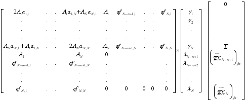 (8)
(8)  does not vary. Matrix of optimisation is developed that is given by Eq. (10).
  (15)
(15) 
 and
and  .
.  for elliptic region
  for hyperbolic region
  for sonic point operator
  for shock point operator
  ,
, 
 (17)
(17)  derivatives can be written as below:
  ,
,  ,
,  ,
, 
 =
= 
 (18)
(18)  , and
, and  .
. 
 (19)
(19) 
 (20)
(20) 
 (21)
(21) 
 (22)
(22) 
 (23)
(23) α0 | Increment factor for CL | CL | CDi | CD=CD0+CDi |
| (ζ/c) max camber in% of chord (bracket shows location in% of chord) | Root washout Values for off-loading Alpha | CL/CDi |
|
| ||||
|---|---|---|---|---|---|---|---|---|---|---|---|---|---|---|
LIF | Before | After | Before | After | Before | After | Before | After | ||||||
2 | NIL | 0.1872 | 0.0065 | 0.0023 | 0.0265 | 0.0223 | 16.32 | 19.40 | 1.36(40%) | 0.0145rad (0.83deg) | 28.8 | 81.39 | 0.849 | 1.027 |
1.2 | 0.2246 | 0.0078 | 0.0033 | 0.0278 | 0.0233 | 17.05 | 20.34 | 1.63(40%) | 0.0104rad (0.59deg) | 28.8 | 68.06 | 0.707 | 0.856 | |
1.4 | 0.2620 | 0.0091 | 0.0046 | 0.0291 | 0.0246 | 17.59 | 20.80 | 1.85(40%) | 0.0063rad (0.36deg) | 28.75 | 56.95 | 0.606 | 0.734 | |
3 | NIL | 0.281 | 0.0147 | 0.0052 | 0.0347 | 0.0252 | 15.27 | 21.03 | 2.0(40%) | 0.0217rad (1.24deg) | 19.11 | 54.04 | 0.849 | 1.028 |
1.1 | 0.309 | 0.0162 | 0.0063 | 0.0362 | 0.0263 | 15.35 | 21.13 | 2.2(40%) | 0.0187rad (1.07deg) | 19.07 | 49.05 | 0.772 | 0.934 | |
1.2 | 0.337 | 0.0176 | 0.0075 | 0.0376 | 0.0275 | 15.44 | 21.11 | 2.37(40%) | 0.0156rad (0.89deg) | 19.14 | 45.00 | 0.707 | 0.856 | |
=0.75, =30, LIF=1.1 | ||||||||
|---|---|---|---|---|---|---|---|---|
|
|
|
|
|
| |||
Before | After | Before | After | Before | After | |||
0.309 | 0.0162 | 0.0063 | 0.2283 | 0.2957 | 0.772 | 0.2988 | 0.3198 | 0.934 |
=0.25, and =250 | ||||||
|---|---|---|---|---|---|---|
=00 | =100 | =150 | ||||
Alpha |
|
|
|
|
|
|
-100 | 0.462 | 0.067 | 0.416 | 0.099 | 0.362 | 0.177 |
-50 | 0.873 | 0.074 | 0.829 | 0.062 | 0.780 | 0.096 |
00 | 1.301 | 0.153 | 1.259 | 0.097 | 1.212 | 0.084 |
50 | 1.754 | 0.310 | 1.712 | 0.207 | 1.669 | 0.146 |
100 | 2.245 | 0.552 | 2.204 | 0.400 | 2.161 | 0.289 |
150 | 2.789 | 0.89 | 2.748 | 0.687 | 2.705 | 0.522 |
=0.25, and =250 | |||||||||
|---|---|---|---|---|---|---|---|---|---|
=00 | =100 | =150 | |||||||
Alpha |
|
|
|
|
|
|
|
|
|
150 | 2.789 | 0.89 | 0.319 | 2.748 | 0.687 | 0.25 | 2.705 | 0.522 | 0.19 |
h/b |
| % change in |
|
|---|---|---|---|
1.0 | 2.748 | - | 0.688 |
0.5 | 2.798 | 1.8% | 0.697 |
0.25 | 2.930 | 4.7% | 0.723 |
0.125 | 3.217 | 9.7% | 0.790 |
0.0625 | 3.799 | 18.0% | 0.947 |
h/b |
|
|
|
|---|---|---|---|
1.0 | -2.298 | - | |
0.5 | -2.338 | -0.040 | 0.002 |
0.25 | -2.443 | -0.105 | 0.009 |
0.125 | -2.671 | -0.228 | 0.041 |
0.0625 | -3.146 | -0.475 | 0.173 |
A | Panel Area |
| Influence Coefficient of jth Panel on ith Control Point |
af | Influence Coefficient of Panels with Fixed Slopes |
b | Span |
c | Local Chord |
ΔCp | Pressure Difference Coefficient |
| Profile Drag Coefficient |
| Induced Drag Coefficient |
| Lift Coefficient |
| Wing Root Bending Moment Coefficient |
| Pitching Moment Coefficient About Wing Apex |
D | Induced Drag |
L | Lift |
| Freestream Mach Number |
M | Local Mach Number |
| Wing Root Bending Moment About Longitudinal Axis |
| Pitching Moment About y Axis |
N | Number of Panels |
U | Freestream Velocity |
w | Downwash |
x,y,z | Chordwise, Spanwise and Vertical Coordinates Respectively |
| Density |
g | Gravitational Constant |
| Angle-of-Attack (Alpha) |
| Velocity Potential Function |
| Circulation Strength of Panels |
| Leading Edge Flap Deflection |
| Trailing Edge Flap Deflection |
i | Control Point of Panel for Collocation of Downwash |
j | Panel Index |
le | Leading Edge |
te | Trailing Edge |
| [1] | Lyu, Z. J.; Martins, J. R. R. A. “Aerodynamic Design Optimization Studies of a Blended-Wing-Body Aircraft”, J. Aircraft. 2014, 51, 1604–1617. |
| [2] | Gupta, S. C., “Computational Algorithms for the Configuration Design,” ICAS Paper No. 98-6.4.5, 21st International Council for the Aeronautical Sciences, September 13-18, 1998, Melbourne, Australia. |
| [3] | Gupta, S. C., “Applied Computational Fluid Dynamics”, Wiley India Pvt. Ltd. 2019. |
| [4] | A. M. Morris, C. B. Allen, T. C. S. Rendall, “CFD based Optimization of airfoils Using Radial Basis Functions for Domain Element Parameterization and Mesh Determination”, Int. J. Numerical Methods Fluids 58(March 2008) 822-860. |
| [5] | Gupta, S. C., “OPSGER: Computer Code for Multi-Constraint Wing Optimisation”, Journal of Aircraft, Vol. 25., No. 6, June 1988. |
| [6] | Alexandar S. Goodman, “Conceptual Aerodynamic Design of Delta-type Tailless Unmanned Aircraft”, International journal of Unmanned Systems Engineering, Vol. 2. No. S2, 2014. |
| [7] | Null, W., and Shkarayev, S., “Effect of Camber on the Aerodynamics of Adaptive-Wing Micro Air Vehicle”, Journal of Aircraft, Vol. 42, No. 6, 2005. |
| [8] | B. K. S. Wood, and J. H. S. Fincham, “Aerodynamic Modelling of the Fish Bone Active Morphing Concept”, Proceeding of RAeS, Applied Aerodynamic Conference, Bristol, UK, June 2014. |
| [9] | J. H. S. Fincham & M. I. Friswell,` `Aerodynamic Optimisation of a Camber Morphing Aerofoil”, Aerospace Science and Technology, Vol. 3, June 2015. |
| [10] | Ahn, J., & Lee, D., “A Computational Study on the Aerodynamic Characteristics of a Flying-Wing MAV design”, 30th AIAA Applied Aerodynamics Conference (2012). |
| [11] | Gupta, S. C., “GENMAP: Computer Code for Mission Adaptive Profile Generation, “Journal of Aircraft, Vol. 25. No. 8, August 1988. |
| [12] | Gupta, S. C., "COPTIM: Computer Code for Canard Coupled Wing Optimization", Canadian Aeronautics and Space Journal, Vol. 37, No. 4, December 1991. |
| [13] | S. C. Gupta, “A Reconstructive Approach for Design of 3-D Low Drag Planar Wings”, Journal of Aerospace Sciences and Technologies: Vol. 72, No. 1, Feb. 2020. |
| [14] | Hummel, D. & Oelker, H. Chr. (1989). Effects of Canard position on the Aerodynamic Characteristics of a Close Coupled Canard Configuration at Low Speed. AGARD-CP-465. |
| [15] | H. L. Atkins and H. A. Hassan, “Transonic Flow Calculations Using Euler Equations”, AIA Journal, Vol. 21, No. 6, June 1983. |
| [16] | Gupta, S. C., “TWING: Computer Code for Transonic Flow Analysis Over Wings”, Presented at the 44 AGM of the Ae. S. I. at I. I. Sc., 11 December 1992, Bangalore. |
| [17] | Gupta, S. C., “Transonic Flow Computations Past Optimally Warped Wings,” ICTACEM – 98, Dec 1-5, 1998, IIT Kharagpur, India. |
| [18] | Mongkol Thianwiboon, “Numerical Aerodynamics Analysis of a Reflexed Aerofoil, N60R, in Ground Effect with Regression Models”, International Journal of Thermofluid Science and Technology, Vol. 9, Issue 1, Paper no. 090105, 2022. |
| [19] | Mongkol Thianwiboon, “A Numerical Comparative Study of the Selected Cambered and Reflexed Aerofoils in Ground Effect”, Engineering Journal, Volume 27, Issue 11, 2023. |
APA Style
Gupta, S. C. (2026). Development of Algorithms and Computer Codes for the Aerodynamic Configurational Design. American Journal of Aerospace Engineering, 12(1), 12-27. https://doi.org/10.11648/j.ajae.20261201.12
ACS Style
Gupta, S. C. Development of Algorithms and Computer Codes for the Aerodynamic Configurational Design. Am. J. Aerosp. Eng. 2026, 12(1), 12-27. doi: 10.11648/j.ajae.20261201.12
@article{10.11648/j.ajae.20261201.12,
  author = {Satish Chander Gupta},
  title = {Development of Algorithms and Computer Codes for the Aerodynamic Configurational Design},
  journal = {American Journal of Aerospace Engineering},
  volume = {12},
  number = {1},
  pages = {12-27},
  doi = {10.11648/j.ajae.20261201.12},
  url = {https://doi.org/10.11648/j.ajae.20261201.12},
  eprint = {https://article.sciencepublishinggroup.com/pdf/10.11648.j.ajae.20261201.12},
  abstract = {Several algorithms and computer codes are developed for the configurational aerodynamic design. Mathematical background, physics involved and their applications are brought out. These range from subsonic to supersonic, including transonic Mach number. Vortex lattice method is applied for handling subsonic and supersonic flow conditions under the linearised flow regime. Finite difference methodology is applied for transonic flow nonlinearities. Matrix of optimization is formed through principles of calculus of variations. The codes developed provide capabilities for inverse design for given loading, aerodynamic drag reduction, high lift to drag designs, generation of morphed profiles, wing optimization in the presence of canard, control surfaces sizing, design of reflex camber wings, and effect of ground proximity on flare manoeuvre, Analysis and Design is made over larger domain of flow field. Details on Camber morphing of wings are elaborated. Camber-morphing aerofoils aim to achieve their camber changes in a smooth way to potentially reduce the drag penalty. Morphing is possible by applying optimisation while restraining variation in camber in certain portions of the wing. A matrix for morphing is developed and scheme so developed is applied herein. Morphing as a concept is also applied to optimise wing for minimum induced drag in the presence of canard, where the slopes of canard camber are made to remain invariant to changes. As the aircraft comes close to ground during landing, runway interferes with aircraft flow field. Some aspects of interference effects of solid boundary wall are established. The influence of wall boundaries on the wing is estimated. Wing is placed at different heights above a horizontal solid surface plane, and an equal opposite vortex system is placed at depth equal to height below this surface. Codes developed find a useful application for design of aircraft for several aspects.},
 year = {2026}
}
TY  - JOUR
T1  - Development of Algorithms and Computer Codes for the Aerodynamic Configurational Design
AU  - Satish Chander Gupta
Y1  - 2026/06/12
PY  - 2026
N1  - https://doi.org/10.11648/j.ajae.20261201.12
DO  - 10.11648/j.ajae.20261201.12
T2  - American Journal of Aerospace Engineering
JF  - American Journal of Aerospace Engineering
JO  - American Journal of Aerospace Engineering
SP  - 12
EP  - 27
PB  - Science Publishing Group
SN  - 2376-4821
UR  - https://doi.org/10.11648/j.ajae.20261201.12
AB  - Several algorithms and computer codes are developed for the configurational aerodynamic design. Mathematical background, physics involved and their applications are brought out. These range from subsonic to supersonic, including transonic Mach number. Vortex lattice method is applied for handling subsonic and supersonic flow conditions under the linearised flow regime. Finite difference methodology is applied for transonic flow nonlinearities. Matrix of optimization is formed through principles of calculus of variations. The codes developed provide capabilities for inverse design for given loading, aerodynamic drag reduction, high lift to drag designs, generation of morphed profiles, wing optimization in the presence of canard, control surfaces sizing, design of reflex camber wings, and effect of ground proximity on flare manoeuvre, Analysis and Design is made over larger domain of flow field. Details on Camber morphing of wings are elaborated. Camber-morphing aerofoils aim to achieve their camber changes in a smooth way to potentially reduce the drag penalty. Morphing is possible by applying optimisation while restraining variation in camber in certain portions of the wing. A matrix for morphing is developed and scheme so developed is applied herein. Morphing as a concept is also applied to optimise wing for minimum induced drag in the presence of canard, where the slopes of canard camber are made to remain invariant to changes. As the aircraft comes close to ground during landing, runway interferes with aircraft flow field. Some aspects of interference effects of solid boundary wall are established. The influence of wall boundaries on the wing is estimated. Wing is placed at different heights above a horizontal solid surface plane, and an equal opposite vortex system is placed at depth equal to height below this surface. Codes developed find a useful application for design of aircraft for several aspects.
VL  - 12
IS  - 1
ER  -
Department of Aeronautical and Aerospace Engineering, Manikudi Venkataraman Jayaraman College of Engineering, Bangalore, India
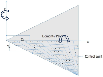
Figure 1. Axis system, paneling scheme and moments.
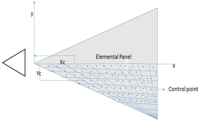
Figure 2. Canard and wing arrangement.
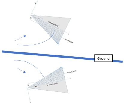
Figure 3. Schematics of wing above the ground and carbon wing (inverted image) below the ground. Arrow indicates the flow direction.
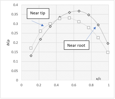
Figure 4. Pressure différence coefficient, optimal surface.=0.75, alpha=30.
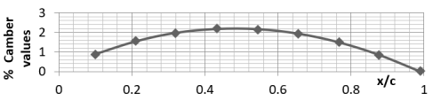
Figure 5. Camber in% of chord at mean aerodynamic chord.
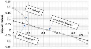
Figure 6. Resulting camber slopes of pre-morphed and morphed Profiles, Mach number is taken as 0.5, alpha=30.
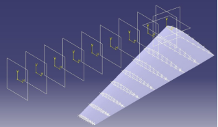
Figure 7. Template of wing developed for max range condition of Jet aircraft.
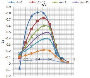
Figure 8. Progressively varying field values of pressure coefficient on upper surface near root, , and Alpha= 40.
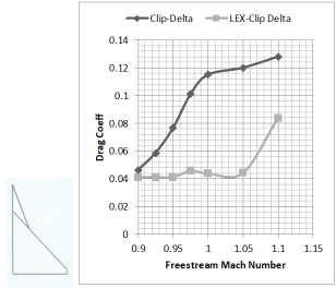
Figure 9. Comparison of Drag Coefficients.
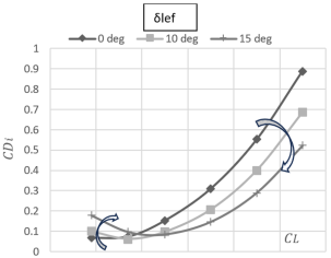
Figure 10. The plot of lift coefficient vrs induced drag coefficient for varied leading edge flap deflections, =0.25 and =250.
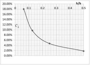
Figure 11. The% increase in lift coefficient during at landing.
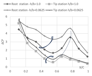
Figure 12. Pressure plots at two different spanwise stations under two extreme heights conditions considered during landing.
Information