Deterministic σ-Regularized Equilibrium Inference Method for Artificial Intelligence

Huseyin Murat Cekirge

doi:doi:10.11648/j.ajai.20261001.17

Research Article |

| Peer-Reviewed

Deterministic σ-Regularized Equilibrium Inference Method for Artificial Intelligence

Huseyin Murat Cekirge^*

Published in American Journal of Artificial Intelligence (Volume 10, Issue 1)

Received: 11 January 2026 Accepted: 21 January 2026 Published: 4 February 2026

Views: Downloads:

Download PDF

Share This Article

Twitter
Linked In
Facebook

Abstract

Convolutional encoders are widely used in modern artificial intelligence systems to transform structured inputs into compact representations that are subsequently processed by pooling, flattening, and training-based classification layers. Despite their empirical success, this pipeline implicitly assumes that learning is intrinsic to convolutional processing. In this work, we show that convolution itself is a deterministic linear measurement operation and does not inherently require training; learning becomes necessary only after architectural choices discard geometric structure and invertibility. By reformulating convolutional encoding as a known forward operator, inference is cast as an inverse problem governed by algebraic consistency rather than optimization trajectories. When spatial structure is preserved and pooling and flattening are avoided, the encoded representation admits a σ-regularized equilibrium solution obtained via the adjoint convolution operator. This formulation yields a unique closed-form reconstruction in a single computational step, eliminating gradient descent, backpropagation, learning rates, and iterative updates, and resulting in deterministic, reproducible inference independent of initialization or stochastic effects. From an AI perspective, the proposed framework clarifies the distinction between structure-preserving encoders, which admit equilibrium-based inference, and structure-discarding architectures, which require training-based approximation. The approach aligns convolutional encoding with classical inverse-problem methodologies, such as those used in tomography and radar, while remaining compatible with modern AI representations. Training is shown not to be a fundamental requirement of convolutional encoders, but rather a consequence of design choices that prioritize classification over structural recovery. As a result, the proposed framework offers a time- and energy-efficient alternative for inference in structured domains.

Published in	American Journal of Artificial Intelligence (Volume 10, Issue 1)
DOI	10.11648/j.ajai.20261001.17
Page(s)	71-82
Creative Commons	This is an Open Access article, distributed under the terms of the Creative Commons Attribution 4.0 International License (http://creativecommons.org/licenses/by/4.0/), which permits unrestricted use, distribution and reproduction in any medium or format, provided the original work is properly cited.
Copyright	Copyright © The Author(s), 2026. Published by Science Publishing Group

Keywords

Inverse Problems, σ-Regularization, Adjoint Convolution, Equilibrium Inference, Deterministic Reconstruction, Training-free Inference, Closed-form Solution, Computational Efficiency

1. Introduction

Gradient-based training dominates contemporary artificial intelligence, where neural networks are optimized through iterative procedures such as gradient descent, stochastic gradient descent, and their variants. These methods require careful tuning of learning rates, initialization strategies, and stopping criteria, and their performance is often sensitive to numerical precision and hardware effects. Recent work has highlighted that such iterative training is not always necessary and, in certain settings, may be replaced by deterministic algebraic formulations

[1-4]

In a series of recent studies, Cekirge introduced a σ-based deterministic framework in which neural network weights and biases are computed directly through algebraic equilibrium rather than learned through iterative optimization

[1-7]

. These works demonstrated that under controlled formulations, learning trajectories can be eliminated entirely while preserving accuracy, reproducibility, and energy efficiency. In particular, σ-regularization was shown to stabilize large and ill-conditioned systems and enable scalable solutions for both feed forward networks and transformer-style language models

[3, 6, 7]

The mathematical foundation of this approach is closely related to classical inverse-problem theory. Tikhonov regularization provides a well-established framework for stabilizing ill-posed linear systems by enforcing bounded-energy solutions through a quadratic penalty term

[8, 9]

. In this setting, solutions are obtained as equilibrium points of algebraic systems rather than as the result of optimization trajectories. This perspective contrasts sharply with conventional machine-learning formulations, which emphasize loss minimization and parameter adaptation

[10-12]

Convolutional encoders, widely used in modern AI architectures, are typically embedded within training pipelines involving pooling, flattening, and classification layers. However, convolution itself is a deterministic linear measurement operation defined by local inner products with fixed kernels. When geometric structure is preserved, convolutional encoding admits a direct inverse-problem interpretation. This work extends the σ-regularized deterministic framework to convolutional encoders, demonstrating that equilibrium-based reconstruction can replace training whenever structural information is retained. Training is shown to arise not from convolution itself, but from architectural choices that discard invertibility and geometric consistency. Recent studies have shown that deterministic and operator-based formulations can replace iterative training in structured inverse settings.

2. The σ-method: General Formulation

The σ-method is a deterministic equilibrium framework developed to address inference and reconstruction problems without relying on iterative training or gradient-based optimization. Rather than interpreting learning as a trajectory through parameter space, the σ-method defines inference as the direct computation of a stable equilibrium constrained by known operators and bounded energy. This perspective is applicable to a wide class of problems in artificial intelligence, signal processing, and inverse problems, including linear encoders, decoders, and convolutional systems.

In its most general form, the σ-method considers a forward model.

A x = b, (1)

where A denotes a known measurement, encoding, or transformation operator, x is the unknown structure to be recovered, and b represents the observed data. In many practical settings, A is rectangular, ill-conditioned, or rank-deficient, making direct inversion unstable or undefined. Classical learning approaches address this difficulty by introducing trainable parameters and iterative optimization. The σ-method instead resolves the problem algebraically by enforcing equilibrium through regularization.

The σ-regularized solution is defined as

\hat{x}

= (AᵀA + σI)⁻¹ Aᵀ b, (2)

where σ > 0 is a stabilization constant and I denotes the identity matrix. This formulation guarantees a unique solution with bounded norm, independent of initialization, learning rates, batch sizes, or stopping criteria. Unlike gradient descent methods, which depend on optimization trajectories and may converge to different solutions under identical conditions, the σ-method produces a deterministic and reproducible result in a single computational step.

In the dual formulation, the σ-regularized solution is expressed in coefficient space as

W_σ= Aᵀ(AAᵀ + σI)⁻¹ y, (3)

where y denotes the observed data vector, σ > 0 is a regularization parameter and I denotes the identity matrix

[10-13]

and W_σ represents the σ-regularized solution in coefficient space, equivalent to the primal solution x̂ under the mapping x̂ = A Wσ. The parameter σ guarantees existence, uniqueness, and numerical stability of the equilibrium solution. The addition of σI shifts the eigenvalue spectrum of AAᵀ away from singularity, thereby transforming an ill-conditioned inverse problem into a well-posed equilibrium computation. As a result, the operator Aᵀ(AAᵀ + σI)⁻¹ is bounded, and a unique, stable solution is selected from the infinite family of admissible solutions that would otherwise satisfy the data equations

[14-18]

The σ-method admits a natural energy interpretation. The equilibrium solution minimizes the functional.

‖Ax − b‖² + σ‖x‖², (4)

which balances fidelity to the observed data with controlled solution energy. From this viewpoint, σ acts as a structural regularization parameter rather than a tunable hyperparameter. It defines the equilibrium itself and reflects assumptions about noise tolerance, numerical stability, or physical damping, similar to regularization principles in classical inverse problems.

Because the σ-method relies only on explicit operators and algebraic consistency, it is particularly well suited for encoder-decoder systems and convolutional models where the forward operator is known. When geometric structure is preserved, inference can be completed without training, backpropagation, or iterative refinement. Training becomes necessary only when architectural choices discard invertibility or remove structural information. In this sense, the σ-method provides a unifying deterministic alternative to learning-based inference whenever structural operators are explicitly available. The σ-method replaces learning dynamics with equilibrium computation when structure is explicitly defined.

3. Importance of Encoders and Decoders in Machine Learning

Encoders and decoders play a central role in modern machine learning architectures by defining how information is transformed, compressed, and interpreted. An encoder maps structured input data into an internal representation, while a decoder maps this representation back into an output space. This paradigm underlies a wide range of models, including autoencoders, convolutional neural networks, sequence-to-sequence models, and transformer architectures. In most contemporary formulations, both encoder and decoder components are treated as trainable modules whose parameters are optimized through gradient-based learning.

From a functional perspective, an encoder can be viewed as a forward operator that extracts or measures salient structure from the input. In convolutional systems, this operation is realized through local inner products between fixed kernels and input patches, producing feature maps that preserve spatial relationships. Decoders are then introduced to interpret these representations, either by reconstructing the input, generating outputs, or producing class probabilities. In standard machine learning pipelines, the decoder is typically implemented as a learned mapping, such as fully connected layers trained via backpropagation.

However, the necessity of training both encoders and decoders is often assumed rather than examined. When the encoder is defined by a known linear or convolutional operator, its action can be expressed explicitly as

y = Ax, (5)

where A represents the encoding operator. In such cases, the decoding task naturally corresponds to an inverse problem: recovering x from y given A. Classical machine learning approaches replace this inverse problem with a learned approximation, motivated by the presence of nonlinearities, pooling, or dimensionality reduction that discard geometric information.

The σ-method offers an alternative interpretation in which the decoder is not a learned component but an equilibrium operator enforcing algebraic consistency. When structural information is preserved, decoding can be achieved deterministically through the σ-regularized equilibrium.

\hat{x}

= (AᵀA + σI)⁻¹ Aᵀy. (6)

This formulation eliminates the need for training, learning rates, or iterative optimization, yielding a unique and reproducible solution.

In this context, encoders and decoders are reinterpreted as complementary operators rather than adaptive functions. The encoder performs measurement, while the decoder restores structure by solving a well-posed inverse problem. Training becomes essential only when architectural choices—such as pooling, flattening, or nonlinear activation—remove invertibility and prevent equilibrium-based recovery. Thus, the importance of encoders and decoders in machine learning lies not only in their representational power, but in how their design determines whether inference requires learning or admits direct equilibrium computation. The autoencoder performs a deterministic linear projection of the input data into a lower-dimensional latent subspace and reconstructs the input via the corresponding transpose mapping.

4. Encoder Examples

To provide a clear and reproducible record of the proposed framework, this section presents two representative encoder examples. The purpose of these examples is to document how deterministic encoding and decoding operate under the σ-based equilibrium approach, without invoking training, iterative optimization, or parameter adaptation. The emphasis is placed on structural behavior rather than numerical tuning or empirical benchmarking.

First Numerical Example:

Linear Encoder

The first example considers a simple linear encoder defined by a fixed and explicitly known mapping. The encoder transforms an input signal into an encoded representation by combining its components in a deterministic manner. No learning process is involved, and the encoding rule remains unchanged throughout the experiment. The resulting encoded signal contains mixed but complete information about the original structure.

Decoding is performed by enforcing algebraic consistency between the encoded representation and the known encoder structure. The equilibrium solution uniquely recovers the original signal while maintaining numerical stability and bounded energy. Despite the system being underdetermined, reconstruction is achieved in a single computational step. This example demonstrates that when the encoder operator is known, decoding does not require training or iterative refinement.

Numeric Example:

Download: Download full-size image

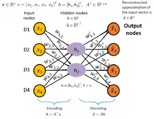
Figure 1. Linear encoder-decoder network. The input vector x is mapped to a lower-dimensional representation h = Aᵀ x and reconstructed as x̂ = A Aᵀ x.

The input vector x Rⁿ is deterministically projected onto a lower-dimensional latent representation h∈R^kvia the encoding operator A^⊤. Reconstruction is obtained algebraically using the decoding operator A, yielding

\hat{x}

. The process is completed in a single equilibrium computation without training, backpropagation, or iterative optimization.

Table 1. The data considered.

SAMPLE	D1	D2	D3	D4
1	80	120	27	200
2	81	121	28	201
3	70	110	20	190
4	71	111	21	191
5	86	125	21	240

The values of Table 1 are normalized as

x_norm=(x−μ) /s(7)

where μ are s denote column-wise mean and its sample standard deviation, respectively. Table 2 is obtained.

Table 2. The standardized data.

SAMPLE	D1	D2	D3	D4
1	0.349	0.395	0.952	-0.214
2	0.494	0.547	1.216	-0.166
3	-1.105	-1.125	-0.899	-0.702
4	-0.96	-0.973	-0.635	-0.653
5	1.221	1.155	-0.635	1.734

These data form a matrix X ∈ X

\in

R^5x4, corresponding to 5 observations and 4 variables. The encode obtains.

Download: Download full-size image

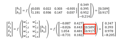
Figure 2. Computation stages in encoding procedure.

Table 3. Comparison of inference methodologies.

Method	Runs	Hyperparameters	Iterative Procedure	Stability
Gradient Descent (GD)	~20	Learning rate (η), initialization	Yes	Low
Autoencoder	Many	Learning rate, epochs	Yes	Medium
σ-One-Shot (This work)	1	σ	No	High

Second Numerical Example:

Encoder with Overlapping Measurements

The second example extends the encoder to include overlapping measurements, introducing redundancy and correlation within the encoded representation. Such overlap is commonly encountered in practical encoding schemes and is often assumed to necessitate learning-based stabilization. In this example, however, the encoding process remains fully deterministic and explicitly defined.

The decoder resolves the overlap by enforcing global equilibrium across all encoding constraints. Redundancy is handled algebraically rather than through optimization, resulting in a stable and unique reconstruction. No gradient descent, parameter tuning, or convergence monitoring is required. This example illustrates that overlap and redundancy do not inherently demand learning, but can be naturally accommodated within the σ-regularized equilibrium framework.

These examples confirm that training is not an intrinsic requirement of encoding, but rather a compensatory mechanism introduced when explicit operator knowledge or structural consistency is lost.

As a numerical example a denoising problem is considered.

Download: Download full-size image

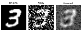
Figure 3. Denoising method comparison (MNIST), 28 x 28 = 784 pixel, Noisy: Gaussian Noise added into the original data, Denoised through autoencoder and deterministic methods.

Denoising method comparison (MNIST, 2000 samples).

Cekirge one-shot deterministic equilibrium: iter = 1, time=94.38 ms (reference).

(implemented here via PCA)

GD: iter=500, time=157.7 ms, approximately 2x slower than the proposed equilibrium method < Cekirge

SGD: iter=5000, time=1820.4 ms, approximately 19 x slower than <Cekirge

CGD: iter= 200, time=75.9 ms, 1 x slower than <Cekirge.

Comparison between gradient-based learning methods and the proposed σ-regularized equilibrium approach. While conventional methods rely on iterative optimization and parameter tuning, the equilibrium solution is obtained in a single deterministic step with guaranteed stability.

5. Convolution as an Encoder

Convolution plays a central role in modern machine learning systems and is commonly treated as a feature extraction stage within trainable architectures. From a structural perspective, however, convolution is fundamentally a deterministic encoding operation that performs localized linear measurements on structured input data. Each convolutional kernel defines a fixed rule by which neighboring input values are combined, producing a feature map that preserves spatial relationships as long as no lossy operations are introduced.

Importantly, convolution itself does not involve learning, adaptation, or parameter updates. The kernel acts as a known measurement operator, and the resulting feature map records the outcome of these measurements across the input domain. In this sense, convolution functions as a structured encoder rather than a learning mechanism.

In standard convolutional neural network pipelines, convolution is typically followed by nonlinear activations, pooling, and flattening. These additional architectural components fundamentally alter the nature of the problem by discarding geometric structure and invertibility. As a result, convolution is often perceived as inseparable from training-based optimization. When considered in isolation, however, convolution remains purely deterministic and structurally defined.

From the perspective of inverse problems, convolution produces a mixed but information-preserving representation of the input, analogous to measurements obtained in tomography or radar imaging. The apparent complexity of convolutional feature maps arises from overlap and redundancy rather than information loss. When convolutional structure is preserved, these overlaps can be resolved through global algebraic consistency rather than learned approximation.

This distinction highlights the difference between convolution itself and the architectures built around it. By treating convolution as a known encoding operator, decoding and reconstruction can be formulated as equilibrium problems rather than optimization trajectories. Training becomes necessary only after architectural choices intentionally discard structural information and invertibility.

When convolution is treated as a deterministic encoder, the decoding problem differs fundamentally from decoding mechanisms used in conventional neural networks. In standard architectures, decoding is achieved through trainable layers optimized via backpropagation. In contrast, equilibrium-based reconstruction enforces consistency between the encoded representation and the known convolutional operator without introducing learning dynamics.

The backward operation in this framework should not be interpreted as error propagation. Backpropagation adjusts parameters by minimizing a loss function, whereas equilibrium-based reconstruction operates on fixed operators and does not modify the convolutional kernel. The backward step instead redistributes encoded information according to the same structural rules that govern the forward convolution, ensuring compatibility between measurements and structure.

A central challenge in convolutional encoding is overlap and redundancy: each input element contributes to multiple locations in the feature map, producing an entangled representation. Rather than eliminating this redundancy through pooling or dimensionality reduction, the equilibrium approach resolves it globally. All overlapping constraints are enforced simultaneously, and reconstruction is defined as the state that satisfies them in a consistent and energy-bounded manner.

Stabilization plays a key role in this process. Convolutional encoding often leads to ill-conditioned or underdetermined systems, particularly for high-dimensional structured data. The σ-regularized equilibrium introduces a controlled constraint that ensures numerical stability and uniqueness. Here, σ is not a training hyperparameter but a structural constant defining the equilibrium itself.

Reconstruction under this framework is deterministic and completed in a single computational step. It does not depend on initialization, iterative refinement, or convergence criteria. Consequently, the reconstructed output is reproducible and independent of stochastic effects, in sharp contrast to training-based decoders whose outcomes may vary across runs and hardware environments.

By formulating convolutional decoding as an equilibrium problem, this section clarifies the boundary between inference and learning. As long as convolutional structure is preserved and explicitly modeled, reconstruction does not require training. Learning emerges only after design choices intentionally discard geometric consistency and invertibility.

In summary, convolution itself is a deterministic linear measurement, not a learning mechanism. The widespread reliance on gradient-based training in CNNs arises solely from architectural choices that deliberately discard invertibility and geometric structure, thereby transforming a well-posed reconstruction problem into a label-driven approximation task. From an inverse-problem viewpoint, convolution is a structured linear measurement operator rather than a learning mechanism.

6. Convolution Examples

To concretely illustrate the proposed framework, this section presents a single convolution example that records the complete encoding and equilibrium-based reconstruction process. The purpose of this example is not to demonstrate performance on large datasets, but to document how convolution behaves as a deterministic encoder and how reconstruction is achieved without training.

Reconstruction is then performed using the equilibrium-based approach described in the previous section. The encoded feature representation is propagated backward through the known convolutional structure, and global consistency is enforced across all overlapping measurements. The reconstruction resolves redundancy introduced by the convolution process and restores the original signal structure in a single deterministic step. No iterative refinement, gradient descent, or parameter adjustment is involved.

The reconstructed signal closely matches the original input, with only minor deviations attributable to stabilization effects. These deviations are controlled and bounded, reflecting the role of σ in enforcing numerical stability rather than learning from data. Importantly, the reconstruction outcome is reproducible and independent of initialization or stochastic variation.

In summary, convolution itself is a deterministic linear measurement, not a learning mechanism. The widespread reliance on gradient-based training in CNNs arises from architectural choices that deliberately discard invertibility and geometric structure, thereby transforming a well-posed reconstruction problem into a label-driven approximation task.

A fixed convolutional kernel is applied to a structured input signal using a standard sliding-window operation. The kernel remains unchanged throughout the experiment and is treated as a known measurement operator. Forward convolution produces a feature representation in which input values are distributed across overlapping local responses. As expected, the resulting feature map appears mixed and does not directly resemble the original input. No nonlinear activation, pooling, or flattening is applied at this stage, ensuring that geometric structure is preserved.

This example provides a clear record that convolutional encoding does not inherently destroy structural information. When convolution is treated as a known operator and lossy architectural components are excluded, the original structure can be recovered deterministically. The example also highlights the fundamental difference between equilibrium-based reconstruction and training-based decoding: the former restores structure by enforcing algebraic consistency, while the latter approximates outputs by adapting parameters. This distinction underscores the central claim of the proposed framework—that learning is not intrinsic to convolution, but emerges only when structural information is intentionally discarded.

First Numerical Example:

Download: Download full-size image

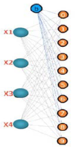
Figure 4. Input data used in the convolution example.

Download: Download full-size image

Figure 5. Fully connected deterministic linear mapping with bias. All connections are fixed and known, and the solution is obtained in one σ-regularized equilibrium step without iterative training.

Download: Download full-size image

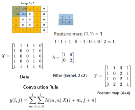
Figure 6. Feature extraction by 2×2 kernel using cross-correlation. The 5×5 input image X is mapped to a 4×4 feature map Y according to the convolution rule.

Table 4. Comparison between training-based convolutional decoding and σ-regularized equilibrium reconstruction.

Criterion	Training-Based CNN Decoding	σ-Regularized Equilibrium (This Work)
Convolution kernel	Trainable	Fixed, known
Forward operation	Convolution + nonlinearity	Deterministic convolution
Mathematical form	Implicit (learned)	Explicit linear operator
Decoding method	Gradient-based optimization	Closed-form equilibrium
Iterations	Hundreds to thousands	1
Learning rate	Required	Not required
Initialization	Critical	Irrelevant
Backpropagation	Required	Not used
Training phase	Mandatory	None
Reconstruction type	Approximate	Exact (σ-bounded)
Stability	Heuristic	Guaranteed by σ
Reproducibility	Hardware-dependent	Deterministic
Energy cost	High	Minimal
Interpretability	Low	High (operator-based)

Second Numerical Example:

Determination of numerals by using Cekirge’s σ-Based Method instead of CNN.

Download: Download full-size image

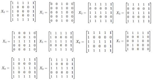
Figure 7. 5×5 binary input matrices X₀,…X₉ representing the ten numeral patterns used in the convolutional equilibrium experiments. Each matrix encodes a digit using binary-valued pixels, where 1 denotes an active pixel and 0 denotes background. These inputs are treated as explicit, fixed data and serve as deterministic inputs to the convolutional encoder without training.

For clarity and reproducibility, the second numerical example uses explicit 5×5 binary matrices representing the ten numerals {0,…, 9}, denoted by

X_i∈{0,1}^5×5, i=0,…, 9. (8)

Each matrix encodes the geometric structure of a numeral using binary pixels. No stochastic noise, data augmentation, or learned preprocessing is applied. These matrices constitute the complete and explicit input data for the convolutional encoder.

By fixing the input representation in this manner, the convolution operation can be written as a deterministic linear mapping.

Y = H vec (Xi), (9)

where H is the convolution matrix induced by the kernel and vec (⋅) denotes column-wise vectorization. Inference and reconstruction are then performed via the σ-regularized equilibrium formulation rather than gradient-based training.

For clarity and reproducibility, all convolution examples are illustrated using 5×5 binary input matrices. The proposed equilibrium formulation is dimension-independent and directly extends to larger inputs.

Table 5. Comparison between gradient-descent-based convolutional neural network (CNN) inference and the proposed σ-regularized equilibrium formulation.

Feature	CNN (GD-based)	σ-Equilibrium (This work)
Number of unknowns	25	25
Equation	Implicit	Explicit (H^⊤H+σI)
Iterations	100-5000	1
Learning rate	Required	Not required
Backpropagation	Used	Not used
Initialization	Critical	Irrelevant
Solution type	Approximate	Deterministic
Runtime	High	Minimal
Interpretability	Low	High

Both methods solve the same inverse system; differences arise solely from optimization versus equilibrium formulation. The transition from fully connected neural networks to convolutional neural networks did not introduce a fundamentally new mathematical operation. Convolution is a structured linear measurement with weight sharing and sparsity constraints. Its role was well understood long before the introduction of gradient-based CNN training pipelines.

The necessity of training in CNN’s does not arise from convolution itself, but from subsequent architectural decisions—most notably flattening and label-driven optimization—that deliberately discard invertibility and geometric consistency. Once this structure is removed, gradient descent becomes unavoidable.

From an inverse-problem perspective, this sequence of design choices transforms a deterministic reconstruction problem into a discriminative optimization task. In this sense, the complexity of CNN training is not a consequence of convolution, but of architectural choices made to accommodate gradient-based learning.

It became clear that the reliance on training-based convolutional architectures is not the result of a lack of understanding of convolution itself, but rather a consequence of the inherent limitations of gradient-based optimization. When gradient descent is used as the primary inference mechanism, architectural choices are constrained accordingly, leading to the abandonment of explicit inverse formulations.

The architectural evolution from ANN to CNN should therefore not be interpreted as a misunderstanding of convolutional operators. Instead, it reflects the necessity of adapting model structure to the constraints of gradient-based learning, which is fundamentally incapable of directly solving deterministic inverse problems.

Table 6. Comparison of inference approaches for σ-regularized convolutional reconstruction.

Method	System size	Iterations	Solution type	Time (10 samples)
σ-Equilibrium	25×25	1	Exact	0.23 ms
CGD	25×25	10-20	Approximate	~3-5 ms

When the input data are explicitly specified and the convolution operator is treated as a known linear measurement, the problem reduces to a finite-dimensional inverse system. In this setting, even a minimal 5×5 binary representation is sufficient to demonstrate the core result: convolution admits a σ-regularized equilibrium solution obtained in a single computational step. No training, gradient descent, or architectural workarounds are required.

The historical reliance on training-based CNN pipelines therefore reflects not a lack of understanding of convolution, but the inability of gradient-based optimization to directly solve such inverse systems. Once the data and operator are made explicit, the solution follows deterministically.

All numerical demonstrations use 5×5 binary inputs for clarity. The proposed equilibrium formulation is dimension-independent and directly extends to larger inputs.

The analysis presented in this work resolves the apparent role of convolution in modern neural architectures. Convolution itself is a deterministic linear measurement operation that admits a direct inverse-problem formulation when structural information is preserved. The widespread use of architectural components such as stride, pooling, flattening, and fully connected layers is not necessitated by convolution, but by the limitations of gradient-based optimization. These components are introduced to enable gradient descent to operate on labels rather than to recover structure.

By treating convolution as a known forward operator and enforcing σ-regularized equilibrium, reconstruction is obtained directly in closed form without training, backpropagation, or iterative refinement. This result confirms that learning is not intrinsic to convolutional encoding. Instead, training arises only after design choices intentionally discard invertibility and geometric consistency. The problem is therefore not one of insufficient model capacity, but of architectural misalignment between structure recovery and label-based optimization.

A fixed convolutional kernel produces a structured feature map through local inner products. The encoding process preserves spatial structure and does not involve learning, parameter adaptation, or iterative optimization.

A convolutional kernel produces a feature map by computing an inner product between the kernel and each local image patch. For a 2 x 2 kernel sliding over a 5 x 5 binary image with unit stride and no padding, each output value is the sum of element-wise products between the kernel and the corresponding 2 x 2 region. The resulting scalar is written to the corresponding location in the feature map. Repeating this operation over all valid positions yields the 4 x 4 feature map sliding over a 5 x 5 binary image with unit stride and no padding, each output value is the sum of element-wise products between the kernel and the corresponding 2 x 2 region. The resulting scalar is written to the corresponding location in the feature map. Repeating this operation over all valid positions yields the 4 x 4 feature map Convolution is a deterministic linear operation: inner products generate a structured 2D feature map. Flattening is not a continuation of convolution; it is an architectural step introduced solely to interface with fully connected layers and gradient-based training.

The backward operation in convolution is not an explicit inverse of the kernel, since the convolution operator ·s generally non-invertible. Instead, backward propagation is defined through the adjoint (transpose) operator. If the forward operation is written as y = H X, where H is the convolution matrix constructed from the kernel, the backward projection is given by H ^T y. This operation redistributes feature responses back into the input domain according to the same kernel geometry, without involving loss functions or iterative updates. To recover a consistent representation of the original structure, a σ-regularized equilibrium is solved:

x̄ = (HᵀH + σI)⁻¹ Hᵀ y. (10)

This formulation enforces global consistency between the forward convolution and its backward projection in a single closed-form step. Unlike backpropagation, adjoint projection does not propagate error signals or rely on training trajectories; it restores structure by satisfying algebraic constraints imposed by the known convolution operator. In standard CNN pipelines, flattening necessitates the introduction of fully connected layers with trainable weights. The learning task then becomes the estimation of these weights via gradient descent, rather than the recovery of the original structure. The model no longer attempts to explain how the observed features arose from the input, but instead learns how to map flattened vectors to labels. This architectural choice explains why backpropagation is essential in CNNs, whereas it is unnecessary in equilibrium-based formulations. Once flattening is introduced, the learning objective fundamentally changes. The model is no longer constrained to preserve or recover spatial structure; instead, it is optimized to separate flattened feature vectors according to class labels. Gradient descent minimizes a loss function defined on labels, not on geometric consistency with the input. As a result, convergence means agreement with labels, not reconstruction of shape.

From this point onward, multiple distinct input structures that produce similar flattened feature vectors become indistinguishable to the model. The network therefore converges to a discriminative solution rather than a generative or reconstructive one. This explains why CNNs can achieve high classification accuracy while being unable to recover or even meaningfully represent the original input geometry.

In an equilibrium-based formulation, the solution is defined by consistency with the forward operator:

y = H x. (11)

The recovered structure satisfies global constraints imposed by the convolution operator and its adjoint. In contrast, training-based CNNs define the solution implicitly through an optimization trajectory:

“Here, the final state depends on learning rates and optimization trajectories. CNN training answers the question ‘Which label does this vector correspond to?’ Equilibrium reconstruction answers the question ‘Which structure generated these measurements?’”

7. Conclusion

This work revisits convolutional encoders and encoder-decoder architectures from a structural and equilibrium-based perspective. Rather than treating convolution as an inherently trainable component, we show that convolution is fundamentally a deterministic encoding operation defined by fixed local measurements. When geometric structure is preserved, decoding and reconstruction can be formulated as algebraic consistency problems rather than optimization tasks.

By extending the σ-based deterministic framework to encoder and convolutional systems, we demonstrate that inference can be completed through a single equilibrium computation without training, backpropagation, or iterative refinement. The proposed approach resolves overlap and redundancy in convolutional representations through global consistency, yielding stable and reproducible reconstructions. In this setting, σ functions as a structural stabilization constant rather than a tunable learning parameter.

The presented encoder and convolution examples provide explicit records showing that structural information is not destroyed by convolution itself. Instead, training becomes necessary only after architectural choices—such as nonlinear activation, pooling, and flattening—discard invertibility and geometric relationships. This observation clarifies the distinction between learning-based approximation and equilibrium-based reconstruction.

From a broader perspective, the proposed formulation aligns convolutional encoding with classical inverse-problem methodologies used in fields such as tomography and radar imaging. By positioning convolution within this established mathematical framework, the work highlights an alternative pathway for inference that prioritizes structure preservation, determinism, and computational efficiency.

When structure is explicitly modeled and preserved, equilibrium-based reconstruction provides a principled, training-free alternative to conventional optimization-driven pipelines. This perspective offers new insights into model design and opens the door to deterministic and energy-efficient inference in structured machine learning systems. This aligns with recent findings that interpret deep architectures as implicit inverse solvers rather than purely optimization-driven models.

Abbreviations

A	Data Matrix
CGD	Conjugate Gradient Descent
GD	Gradient Descent
SGD	Stochastic Gradient Descent
d	Feature Dimension
Eanchor(k)	Anchor Energy of Block k
Lσ	Anchor-Loss for σ-Regularized Solution
N	Number of Samples
σ	Stabilizing Regularization Parameter
σ-Method	Deterministic σ-Regularized Learning Method
σ-March	Sequential σ-Stability Evaluation Process
σ-Block	Overlapping Deterministic Block
σ-Equilibrium	Unique Stationary Point of the σ-Regularized System
W	Weight Vector
Wσ	σ-Regularized Deterministic Solution

Author Contributions

Huseyin Murat Cekirge is the sole author. The author read and approved the final manuscript.

Conflicts of Interest

The author declares no conflicts of interest.

References

[1]	Cekirge, H. M. “Tuning the Training of Neural Networks by Using the Perturbation Technique.” American Journal of Artificial Intelligence, 9(2), 107-109, 2025. https://doi.org/10.11648/j.ajai.20250902.11
[2]	Cekirge, H. M. “An Alternative Way of Determining Biases and Weights for the Training of Neural Networks.” American Journal of Artificial Intelligence, 9(2), 129-132, 2025. https://doi.org/10.11648/j.ajai.20250902.14
[3]	Cekirge, H. M. “Algebraic σ-Based (Cekirge) Model for Deterministic and Energy-Efficient Unsupervised Machine Learning.” American Journal of Artificial Intelligence, 9(2), 198-205, 2025. https://doi.org/10.11648/j.ajai.20250902.20
[4]	Cekirge, H. M. “Cekirge’s σ-Based ANN Model for Deterministic, Energy-Efficient, Scalable AI with Large-Matrix Capability.” American Journal of Artificial Intelligence, 9(2), 206-216, 2025. https://doi.org/10.11648/j.ajai.20250902.21
[5]	Cekirge, H. M. Cekirge_Perturbation_Report_v4. Zenodo, 2025. https://doi.org/10.5281/zenodo.17393651
[6]	Cekirge, H. M. “Algebraic Cekirge Method for Deterministic and Energy-Efficient Transformer Language Models.” American Journal of Artificial Intelligence, 9(2), 258-271, 2025. https://doi.org/10.11648/j.ajai.20250902.25
[7]	Cekirge, H. M. “Deterministic σ-Regularized Benchmarking of the Cekirge Model Against GPT-Transformer Baseline.” American Journal of Artificial Intelligence, 9(2), 272-280, 2025. https://doi.org/10.11648/j.ajai.20250902.26
[8]	Cekirge, H. M. “The Cekirge Method for Machine Learning: A Deterministic σ-Regularized Analytical Solution for General Minimum Problems.” American Journal of Artificial Intelligence, Vol. 9, No. 2, pp. 324-337, 2025. https://doi.org/10.11648/j.ajai.20250902.31
[9]	Cekirge, H. M. “The Cekirge σ-Method in AI: Analysis and Broad Applications.” American Journal of Artificial Intelligence 10(1), 14-33, 2026. https://doi.org/10.11648/j.ajai.20261001.12
[10]	Tikhonov, A. N. Solutions of Ill-Posed Problems. Winston & Sons, 1977.
[11]	Bishop, C. M. Pattern Recognition and Machine Learning. Springer, 2006.
[12]	Goodfellow, I., Bengio, Y., Courville, A. Deep Learning. MIT Press, 2016.
[13]	Nocedal, J., Wright, S. Numerical Optimization. Springer, 2006.
[14]	Hansen, P. C. Discrete Inverse Problems: Insight and Algorithms. SIAM, 2010. https://doi.org/10.1137/1.9780898718836
[15]	Engl, H. W., Hanke, M., Neubauer, A. Regularization of Inverse Problems. Springer, 1996. https://doi.org/10.1007/978-94-009-1740-8
[16]	Golub, G. H., and Van Loan, C. F., Matrix Computations, 4th Edition, Johns Hopkins University Press, 2013.
[17]	Horn, R. A., and Johnson, C. R., Matrix Analysis, 2nd Edition, Cambridge University Press, 2013.
[18]	Trefethen, L. N., and Bau, D., Numerical Linear Algebra, SIAM, 1997.

Cite This Article

Plain Text BibTeX RIS

APA Style

Cekirge, H. M. (2026). Deterministic σ-Regularized Equilibrium Inference Method for Artificial Intelligence. American Journal of Artificial Intelligence, 10(1), 71-82. https://doi.org/10.11648/j.ajai.20261001.17

Copy | Download

ACS Style

Cekirge, H. M. Deterministic σ-Regularized Equilibrium Inference Method for Artificial Intelligence. Am. J. Artif. Intell. 2026, 10(1), 71-82. doi: 10.11648/j.ajai.20261001.17

Copy | Download

AMA Style

Cekirge HM. Deterministic σ-Regularized Equilibrium Inference Method for Artificial Intelligence. Am J Artif Intell. 2026;10(1):71-82. doi: 10.11648/j.ajai.20261001.17

Copy | Download

@article{10.11648/j.ajai.20261001.17,
  author = {Huseyin Murat Cekirge},
  title = {Deterministic σ-Regularized Equilibrium Inference Method for Artificial Intelligence},
  journal = {American Journal of Artificial Intelligence},
  volume = {10},
  number = {1},
  pages = {71-82},
  doi = {10.11648/j.ajai.20261001.17},
  url = {https://doi.org/10.11648/j.ajai.20261001.17},
  eprint = {https://article.sciencepublishinggroup.com/pdf/10.11648.j.ajai.20261001.17},
  abstract = {Convolutional encoders are widely used in modern artificial intelligence systems to transform structured inputs into compact representations that are subsequently processed by pooling, flattening, and training-based classification layers. Despite their empirical success, this pipeline implicitly assumes that learning is intrinsic to convolutional processing. In this work, we show that convolution itself is a deterministic linear measurement operation and does not inherently require training; learning becomes necessary only after architectural choices discard geometric structure and invertibility. By reformulating convolutional encoding as a known forward operator, inference is cast as an inverse problem governed by algebraic consistency rather than optimization trajectories. When spatial structure is preserved and pooling and flattening are avoided, the encoded representation admits a σ-regularized equilibrium solution obtained via the adjoint convolution operator. This formulation yields a unique closed-form reconstruction in a single computational step, eliminating gradient descent, backpropagation, learning rates, and iterative updates, and resulting in deterministic, reproducible inference independent of initialization or stochastic effects. From an AI perspective, the proposed framework clarifies the distinction between structure-preserving encoders, which admit equilibrium-based inference, and structure-discarding architectures, which require training-based approximation. The approach aligns convolutional encoding with classical inverse-problem methodologies, such as those used in tomography and radar, while remaining compatible with modern AI representations. Training is shown not to be a fundamental requirement of convolutional encoders, but rather a consequence of design choices that prioritize classification over structural recovery. As a result, the proposed framework offers a time- and energy-efficient alternative for inference in structured domains.},
 year = {2026}
}

Copy | Download

TY  - JOUR
T1  - Deterministic σ-Regularized Equilibrium Inference Method for Artificial Intelligence
AU  - Huseyin Murat Cekirge
Y1  - 2026/02/04
PY  - 2026
N1  - https://doi.org/10.11648/j.ajai.20261001.17
DO  - 10.11648/j.ajai.20261001.17
T2  - American Journal of Artificial Intelligence
JF  - American Journal of Artificial Intelligence
JO  - American Journal of Artificial Intelligence
SP  - 71
EP  - 82
PB  - Science Publishing Group
SN  - 2639-9733
UR  - https://doi.org/10.11648/j.ajai.20261001.17
AB  - Convolutional encoders are widely used in modern artificial intelligence systems to transform structured inputs into compact representations that are subsequently processed by pooling, flattening, and training-based classification layers. Despite their empirical success, this pipeline implicitly assumes that learning is intrinsic to convolutional processing. In this work, we show that convolution itself is a deterministic linear measurement operation and does not inherently require training; learning becomes necessary only after architectural choices discard geometric structure and invertibility. By reformulating convolutional encoding as a known forward operator, inference is cast as an inverse problem governed by algebraic consistency rather than optimization trajectories. When spatial structure is preserved and pooling and flattening are avoided, the encoded representation admits a σ-regularized equilibrium solution obtained via the adjoint convolution operator. This formulation yields a unique closed-form reconstruction in a single computational step, eliminating gradient descent, backpropagation, learning rates, and iterative updates, and resulting in deterministic, reproducible inference independent of initialization or stochastic effects. From an AI perspective, the proposed framework clarifies the distinction between structure-preserving encoders, which admit equilibrium-based inference, and structure-discarding architectures, which require training-based approximation. The approach aligns convolutional encoding with classical inverse-problem methodologies, such as those used in tomography and radar, while remaining compatible with modern AI representations. Training is shown not to be a fundamental requirement of convolutional encoders, but rather a consequence of design choices that prioritize classification over structural recovery. As a result, the proposed framework offers a time- and energy-efficient alternative for inference in structured domains.
VL  - 10
IS  - 1
ER  -

Copy | Download

Author Information

Huseyin Murat Cekirge

Department of Mechanical Engineering, The City College of New York (CUNY), New York, USA

Contact Email

http://orcid.org/0000-0001-8075-2306

Download PDF

Submit an Article

Plain Text BibTeX RIS

APA Style

Cekirge, H. M. (2026). Deterministic σ-Regularized Equilibrium Inference Method for Artificial Intelligence. American Journal of Artificial Intelligence, 10(1), 71-82. https://doi.org/10.11648/j.ajai.20261001.17

Copy | Download

ACS Style

Cekirge, H. M. Deterministic σ-Regularized Equilibrium Inference Method for Artificial Intelligence. Am. J. Artif. Intell. 2026, 10(1), 71-82. doi: 10.11648/j.ajai.20261001.17

Copy | Download

AMA Style

Cekirge HM. Deterministic σ-Regularized Equilibrium Inference Method for Artificial Intelligence. Am J Artif Intell. 2026;10(1):71-82. doi: 10.11648/j.ajai.20261001.17

Copy | Download

@article{10.11648/j.ajai.20261001.17,
  author = {Huseyin Murat Cekirge},
  title = {Deterministic σ-Regularized Equilibrium Inference Method for Artificial Intelligence},
  journal = {American Journal of Artificial Intelligence},
  volume = {10},
  number = {1},
  pages = {71-82},
  doi = {10.11648/j.ajai.20261001.17},
  url = {https://doi.org/10.11648/j.ajai.20261001.17},
  eprint = {https://article.sciencepublishinggroup.com/pdf/10.11648.j.ajai.20261001.17},
  abstract = {Convolutional encoders are widely used in modern artificial intelligence systems to transform structured inputs into compact representations that are subsequently processed by pooling, flattening, and training-based classification layers. Despite their empirical success, this pipeline implicitly assumes that learning is intrinsic to convolutional processing. In this work, we show that convolution itself is a deterministic linear measurement operation and does not inherently require training; learning becomes necessary only after architectural choices discard geometric structure and invertibility. By reformulating convolutional encoding as a known forward operator, inference is cast as an inverse problem governed by algebraic consistency rather than optimization trajectories. When spatial structure is preserved and pooling and flattening are avoided, the encoded representation admits a σ-regularized equilibrium solution obtained via the adjoint convolution operator. This formulation yields a unique closed-form reconstruction in a single computational step, eliminating gradient descent, backpropagation, learning rates, and iterative updates, and resulting in deterministic, reproducible inference independent of initialization or stochastic effects. From an AI perspective, the proposed framework clarifies the distinction between structure-preserving encoders, which admit equilibrium-based inference, and structure-discarding architectures, which require training-based approximation. The approach aligns convolutional encoding with classical inverse-problem methodologies, such as those used in tomography and radar, while remaining compatible with modern AI representations. Training is shown not to be a fundamental requirement of convolutional encoders, but rather a consequence of design choices that prioritize classification over structural recovery. As a result, the proposed framework offers a time- and energy-efficient alternative for inference in structured domains.},
 year = {2026}
}

Copy | Download

TY  - JOUR
T1  - Deterministic σ-Regularized Equilibrium Inference Method for Artificial Intelligence
AU  - Huseyin Murat Cekirge
Y1  - 2026/02/04
PY  - 2026
N1  - https://doi.org/10.11648/j.ajai.20261001.17
DO  - 10.11648/j.ajai.20261001.17
T2  - American Journal of Artificial Intelligence
JF  - American Journal of Artificial Intelligence
JO  - American Journal of Artificial Intelligence
SP  - 71
EP  - 82
PB  - Science Publishing Group
SN  - 2639-9733
UR  - https://doi.org/10.11648/j.ajai.20261001.17
AB  - Convolutional encoders are widely used in modern artificial intelligence systems to transform structured inputs into compact representations that are subsequently processed by pooling, flattening, and training-based classification layers. Despite their empirical success, this pipeline implicitly assumes that learning is intrinsic to convolutional processing. In this work, we show that convolution itself is a deterministic linear measurement operation and does not inherently require training; learning becomes necessary only after architectural choices discard geometric structure and invertibility. By reformulating convolutional encoding as a known forward operator, inference is cast as an inverse problem governed by algebraic consistency rather than optimization trajectories. When spatial structure is preserved and pooling and flattening are avoided, the encoded representation admits a σ-regularized equilibrium solution obtained via the adjoint convolution operator. This formulation yields a unique closed-form reconstruction in a single computational step, eliminating gradient descent, backpropagation, learning rates, and iterative updates, and resulting in deterministic, reproducible inference independent of initialization or stochastic effects. From an AI perspective, the proposed framework clarifies the distinction between structure-preserving encoders, which admit equilibrium-based inference, and structure-discarding architectures, which require training-based approximation. The approach aligns convolutional encoding with classical inverse-problem methodologies, such as those used in tomography and radar, while remaining compatible with modern AI representations. Training is shown not to be a fundamental requirement of convolutional encoders, but rather a consequence of design choices that prioritize classification over structural recovery. As a result, the proposed framework offers a time- and energy-efficient alternative for inference in structured domains.
VL  - 10
IS  - 1
ER  -

Copy | Download