Abstract
Breast cancer is a major health concern, and early detection can make a great difference in treatment and survival rates for breast cancer patients. Machine learning methods have noticeably improved prediction accuracy on high-dimensional medical datasets and have become widely used tools in medical diagnostics. The transition to a quantum computational framework has opened new directions in machine learning research. By using qubits instead of classical bits, quantum models may provide new ways to represent and process complex medical data. In medical diagnostics, this has led to a growing interest in whether quantum approaches can improve classification performance more effectively than classical methods. The purpose of this paper is to compare classical and quantum machine learning models on the task of breast cancer classification and to determine whether quantum models can achieve higher accuracy and faster prediction on a selected dataset. Alongside the main simulator-based experiment, a smaller experiment was performed on a real IBM quantum computer to demonstrate the practical execution of the same task under current hardware constraints. In the practical part of the study, the Wisconsin Diagnostic Breast Cancer (WDBC) dataset was used. This dataset consists of 569 samples with 30 numerical features extracted from digitized fine needle aspirate images and provides a reliable basis for evaluating model performance. A comparative analysis was conducted between classical and quantum machine learning models, including a support vector machine (SVM), an artificial neural network (ANN), a quantum support vector machine (QSVM), and a hybrid quantum-classical neural network (QNN). In the simulator-based experiment, both SVM and ANN achieved an accuracy of 0.956 with an F1-score of 0.965 on the test set, while QSVM reached an accuracy of 0.807 with an F1-score of 0.866 and the Hybrid QNN achieved 0.623 accuracy with an F1-score of 0.677. These quantum and hybrid models also required substantially longer training times than the classical baselines. A small hardware experiment on an IBM quantum device further illustrates both the practical feasibility and the current limitations of executing this classification task on noisy intermediate-scale quantum hardware.
Keywords
Quantum Machine Learning, Quantum Computing, WDBC Dataset, Support Vector Machine,
Hybrid Quantum‑classical Neural Network
1. Introduction
Technological progress nowadays is largely driven by two rapidly advancing fields - artificial intelligence and quantum computing
| [1] | R. Ghosh and S. Doss, “Shaping tomorrow: The convergence of Artificial General Intelligence and Quantum Computing,” in Interplay of Artificial General Intelligence with Quantum Computing. Sustainable Artificial Intelligence-Powered Applications, C. K. K. Reddy, S. Joseph, H. Joshi, M. Ouaissa, and M. M. Hanafiah, Eds. Springer, Cham, 2025, pp. 1-10,
https://doi.org/10.1007/978-3-031-87931-9_1 |
[1]
.
Artificial intelligence (AI) is concerned with creating computer systems that can learn from data, recognize patterns and support decision making. In practice, these systems keep improving as they receive more data and as learning algorithms are refined
| [1] | R. Ghosh and S. Doss, “Shaping tomorrow: The convergence of Artificial General Intelligence and Quantum Computing,” in Interplay of Artificial General Intelligence with Quantum Computing. Sustainable Artificial Intelligence-Powered Applications, C. K. K. Reddy, S. Joseph, H. Joshi, M. Ouaissa, and M. M. Hanafiah, Eds. Springer, Cham, 2025, pp. 1-10,
https://doi.org/10.1007/978-3-031-87931-9_1 |
| [3] | NASA, “What is Artificial Intelligence ?,” NASA, May 13, 2024. Available:
https://www.nasa.gov/what-is-artificial-intelligence/
(Accessed: Mar. 2026). |
[1, 3]
.
Machine learning is a subfield of artificial intelligence in which computer systems learn from data. In computer systems, experience exists in the form of data
| [4] | G. Acampora, A. Ambainis, N. Ares, L. Banchi, P. Bhardwaj, D. Binosi, G. A. D. Briggs, T. Calarco, V. Dunjko, J. Eisert, O. Ezratty, P. Erker, F. Fedele, E. Gil-Fuster, M. Gärttner, M. Granath, M. Heyl, I. Kerenidis, M. Klusch, A. F. Kockum, R. Kueng, M. Krenn, J. Lässig, A. Macaluso, S. Maniscalco, F. Marquardt, K. Michielsen, G. Muñoz-Gil, D. Müssig, H. P. Nautrup, S. A. Neubauer, E. van Nieuwenburg, R. Orus, J. Schmiedmayer, M. Schmitt, P. Slusallek, F. Vicentini, C. Weitenberg, and F. K. Wilhelm, “Quantum computing and artificial intelligence: status and perspectives,” arXiv [quant-ph], 2025,
https://doi.org/10.48550/arXiv.2505.23860 |
[4]
. The main task of ML is to create models by training learning algorithms to make predictions or decisions based on that data
| [2] | C. Stryker and E. Kavlakoglu, “What Is Artificial Intelligence ?,” IBM Think, IBM, 2024. Available:
https://www.ibm.com/think/topics/artificial-intelligence
(Accessed: Mar. 2026). |
| [4] | G. Acampora, A. Ambainis, N. Ares, L. Banchi, P. Bhardwaj, D. Binosi, G. A. D. Briggs, T. Calarco, V. Dunjko, J. Eisert, O. Ezratty, P. Erker, F. Fedele, E. Gil-Fuster, M. Gärttner, M. Granath, M. Heyl, I. Kerenidis, M. Klusch, A. F. Kockum, R. Kueng, M. Krenn, J. Lässig, A. Macaluso, S. Maniscalco, F. Marquardt, K. Michielsen, G. Muñoz-Gil, D. Müssig, H. P. Nautrup, S. A. Neubauer, E. van Nieuwenburg, R. Orus, J. Schmiedmayer, M. Schmitt, P. Slusallek, F. Vicentini, C. Weitenberg, and F. K. Wilhelm, “Quantum computing and artificial intelligence: status and perspectives,” arXiv [quant-ph], 2025,
https://doi.org/10.48550/arXiv.2505.23860 |
[2, 4]
. Machine learning methods are used in many areas, including medicine, finance and industry, where they recognize patterns, make predictions and support decision making
. Still, there are several limitations to this technique. It usually needs well labeled data, and sometimes a model can memorize the training examples and then make mistakes on new cases. Besides that, trained models can be hard to explain in simple terms, and there can be serious financial or practical consequences if they accidentally learn and repeat unfair patterns that already exist in the data
.
By replacing bits with qubits, powerful quantum particles, the development of quantum computing began. Quantum computing, which is based on the basic principles of quantum mechanics, introduces new possibilities for artificial intelligence and therefore for machine learning. Superposition, quantum entanglement, quantum interference and quantum parallelism can accelerate the optimization processes, make it possible to work with very large datasets, and reduce the complexity of the search problem.
The main goal of this study is to compare classical and quantum machine learning models on a clinically relevant breast cancer dataset and to show, based on the obtained results, which models perform better and run faster in this specific setting. In addition, a small demonstration test is carried out on a real quantum computer to show that, under current hardware constraints, the same task can already be executed on real quantum hardware.
2. Theoretical Background
Quantum computing has created a completely new paradigm in the computing world
| [1] | R. Ghosh and S. Doss, “Shaping tomorrow: The convergence of Artificial General Intelligence and Quantum Computing,” in Interplay of Artificial General Intelligence with Quantum Computing. Sustainable Artificial Intelligence-Powered Applications, C. K. K. Reddy, S. Joseph, H. Joshi, M. Ouaissa, and M. M. Hanafiah, Eds. Springer, Cham, 2025, pp. 1-10,
https://doi.org/10.1007/978-3-031-87931-9_1 |
[1]
. It represents a large interdisciplinary field at the intersection of quantum physics, mathematics and computing. Using the main concepts of quantum mechanics, quantum computing aims to provide new ways of solving problems that are difficult for traditional computers to solve
.
The simultaneous processing of huge amounts of data using quantum phenomena such as superposition, entanglement, and tunneling has made significant advances in materials science, optimization, and cryptography
| [1] | R. Ghosh and S. Doss, “Shaping tomorrow: The convergence of Artificial General Intelligence and Quantum Computing,” in Interplay of Artificial General Intelligence with Quantum Computing. Sustainable Artificial Intelligence-Powered Applications, C. K. K. Reddy, S. Joseph, H. Joshi, M. Ouaissa, and M. M. Hanafiah, Eds. Springer, Cham, 2025, pp. 1-10,
https://doi.org/10.1007/978-3-031-87931-9_1 |
[1]
. This combination of quantum physics and computer science represents a major technological revolution of the 21st century.
Quantum computing, although still in development, is slowly establishing a new and more powerful basis for information processing
.
The same parallel processing that allows quantum computers to work in material science, optimization, and cryptography suggests that, in the future, quantum computing is expected to efficiently simulate many relevant physical processes, under certain conditions
.
2.1. Quantum Particles (Qubits)
At the heart of a quantum system is a quantum particle, a
qubit. Unlike traditional computing systems where information is represented as the digits 0 or 1, quantum computers can be in a superposition of these states simultaneously. Calculations that would normally have to be performed separately with 0 or 1 on a classical computer could now be performed in a single operation using qubits on a quantum computer. It is important to understand that although a qubit can be both 0 and 1 at the same time, when a qubit is measured, the result of the measurement is only one of two classical states, either 0 or 1
| [10] | C. Hughes, J. Isaacson, A. Perry, R. F. Sun, and J. Turner, “What Is a Qubit ?,” in Quantum Computing for the Quantum Curious, Cham: Springer International Publishing, 2021, pp. 7-16, https://doi.org/10.1007/978-3-030-61601-4_2 |
| [27] | M. Schuld, I. Sinayskiy, and F. Petruccione, “An introduction to quantum machine learning,” Contemp. Phys., vol. 56, no. 2, pp. 172-185, 2015, https://doi.org/10.1080/00107514.2014.964942 |
| [30] | M. Schuld and F. Petruccione, Supervised Learning with Quantum Computers. Cham: Springer, 2018, in Quantum Science and Technology, https://doi.org/10.1007/978-3-319-96424-9 |
[10, 27, 30]
.
That's why we call quantum systems two-state, because to describe the system, we must have two measurable states, which in this case are 0 and 1
| [6] | M. A. Nielsen and I. L. Chuang, Quantum Computation and Quantum Information, 10th Anniversary ed. Cambridge, U.K.: Cambridge University Press, 2010,
https://doi.org/10.1017/CBO9780511976667 |
| [27] | M. Schuld, I. Sinayskiy, and F. Petruccione, “An introduction to quantum machine learning,” Contemp. Phys., vol. 56, no. 2, pp. 172-185, 2015, https://doi.org/10.1080/00107514.2014.964942 |
[6, 27]
.
In practice, a qubit can be realized in many different ways, depending on the technology. A qubit can be carried by a single atom, which has internal energy states that can be prepared and controlled using lasers or electromagnetic fields. A system can be made using a single electron, whose spin (up or down) serves as the two basic states |0⟩ and |1⟩. A qubit can also be represented by a single photon, a particle of light. The polarization or the path of the photon encodes the quantum information. More complex quantum systems are realised using more complex physical systems like superconducting circuits or quantum dots which are engineered to behave like a two level quantum system
.
2.2. Fundamental Quantum Phenomena
Superposition allows a qubit to be in a both states simultaneously. This is a key property of a quantum particle and it is a real power of quantum systems. Superposition enables the exploration of many possible solutions in parallel, which is crucial for accelerating complex algorithms
| [8] | N. S. Yanofsky and M. A. Mannucci, Quantum Computing for Computer Scientists, Cambridge, Cambridge University Press, 2008, https://doi.org/10.1017/CBO9780511813887 |
| [42] | K. Zaman, A. Marchisio, M. A. Hanif, and M. Shafique, “A Survey on Quantum Machine Learning: Basics, Current Trends, Challenges, Opportunities, and the Road Ahead,” arXiv [quant-ph], 2023, https://doi.org/10.48550/arXiv.2310.10315 |
[8, 42]
.
To understand quantum superposition, we can think of a coin. A coin can land as heads or tails. The probability for each state is equal to 50%. While the coin is in the air it is not heads or tails, it is both. When it lands there is just one result, heads or tails. The word state means the way a system can be at a specific time. The coin is either a heads state or tails state, but when it is still in the air, it can be a mixed state of both. All of these are the possible states of coin system. During the flip, a coin exists in superposition. Observing it, collapses this superposition to one or the other state, heads or tails, chosen at random with a certain probability. This is a measurement that destroys superposition. A quantum system can have many states at the same time
| [10] | C. Hughes, J. Isaacson, A. Perry, R. F. Sun, and J. Turner, “What Is a Qubit ?,” in Quantum Computing for the Quantum Curious, Cham: Springer International Publishing, 2021, pp. 7-16, https://doi.org/10.1007/978-3-030-61601-4_2 |
| [42] | K. Zaman, A. Marchisio, M. A. Hanif, and M. Shafique, “A Survey on Quantum Machine Learning: Basics, Current Trends, Challenges, Opportunities, and the Road Ahead,” arXiv [quant-ph], 2023, https://doi.org/10.48550/arXiv.2310.10315 |
[10, 42]
.
Quantum entanglement is a unique phenomenon in which two quantum systems are so deeply connected that to learn something about one system, you will immediately learn something about the other, no matter how far apart they are. A measurement made on one system immediately affects the state of the other. However, any quantum bit in the world of quantum computers can exist in an entangled state. This means that the states of these qubits cannot be described separately, but only work together as an indivisible whole. This unique ability of entangled qubits adds depth to the concept of quantum computing and allows parallel computations, providing speed and efficiency that no classical computer can achieve on specific sets of complex problems such as factoring large numbers or searching unstructured databases
.
Unlike classical computers, which use logic gates to perform algorithms, quantum computers have a quantum analogue and use
quantum logic gates. These are quantum versions of classical gates, which act on qubits instead of classical bits, and they can be implemented using different physical technologies to create a real quantum system. For example, quantum gates can be realized using superconducting materials on silicon or sapphire chips, photons guided through optical circuits, or trapped ion technologies, where individual atoms are controlled with lasers
. Mathematically, they are expressed as a unitary operator acting on qubit states. This unitary is marked as a quantum gate that respects unitarity, expressed by:
where U is the respective gate matrix and U† its adjoint, what guarantees that the related evolution is not irreversible. A reversible operation is one that allows the final state to uniquely identify the initial state, implying no information about the input has been lost and so in principle the computation can be run backwards to recover it. Single-qubit gates include Pauli-X, Pauli-Y, Pauli-Z, rotation (over X, Y and Z-axis), Hadamard gate. Multi-qubit gates, like controlled-NOT (CNOT) gate can create entanglement between qubits
| [42] | K. Zaman, A. Marchisio, M. A. Hanif, and M. Shafique, “A Survey on Quantum Machine Learning: Basics, Current Trends, Challenges, Opportunities, and the Road Ahead,” arXiv [quant-ph], 2023, https://doi.org/10.48550/arXiv.2310.10315 |
[42]
. In each case, the gates manipulate the quantum states in a way that allows the quantum computer to run algorithms on large datasets and perform operations that are difficult for classical computers
| [10] | C. Hughes, J. Isaacson, A. Perry, R. F. Sun, and J. Turner, “What Is a Qubit ?,” in Quantum Computing for the Quantum Curious, Cham: Springer International Publishing, 2021, pp. 7-16, https://doi.org/10.1007/978-3-030-61601-4_2 |
[10]
.
2.3. Machine Learning Vs. Quantum Machine Learning
Machine learning (ML) is a branch in artificial intelligence, where algorithms become better at their jobs by learning from data instead of having human experts tell them exactly how to perform each task. Contrary to explicitly programming every stage of a solution, an ML system infers a model from input-output examples and can be especially useful when the problem in fact cannot easily be formalized, or expert knowledge is limited but large datasets are available. A prime example is face recognition. Instead of programming how to detect, describe, and compare facial features, we supply a large corpus of labeled images and allow the learning algorithm to find its own mapping from images to identities
| [13] | A. A. Torres‑García, C. A. Reyes‑Garcia, L. Villaseñor‑Pineda, and O. Mendoza‑Montoya, Eds., Biosignal Processing and Classification Using Computational Learning and Intelligence: Principles, Algorithms, and Applications. Academic Press, 2021. |
| [14] | M. W. Berry, A. Mohamed, and B. W. Yap, Eds., Supervised and Unsupervised Learning for Data Science. Cham: Springer, 2020. https://doi.org/10.1007/978-3-030-22475-2 |
[13, 14]
.
Sitting between AI and statistics, ML is focused on how to bring structure out of data so that we can interpret novel or unseen inputs. In practice, ML methods are applied to tasks that come naturally to humans. For example, identifying objects in images or speech or patterns in a time series or optimizing strategies for making decisions, but are clumsy to articulate as formal sets of rules. These advances have made it possible to directly apply ML systems across many domains like healthcare, finance, logistics and cybersecurity
| [27] | M. Schuld, I. Sinayskiy, and F. Petruccione, “An introduction to quantum machine learning,” Contemp. Phys., vol. 56, no. 2, pp. 172-185, 2015, https://doi.org/10.1080/00107514.2014.964942 |
| [42] | K. Zaman, A. Marchisio, M. A. Hanif, and M. Shafique, “A Survey on Quantum Machine Learning: Basics, Current Trends, Challenges, Opportunities, and the Road Ahead,” arXiv [quant-ph], 2023, https://doi.org/10.48550/arXiv.2310.10315 |
[27, 42]
.
The explosive growth and presence of ML in the past few years can be traced back to a number of converging trends: massive datasets available for training, continuing improvements in hardware providing more memory and faster processors, free open source software lowering the barrier to experimentation on your own machine, and substantial investment from industry and government
| [13] | A. A. Torres‑García, C. A. Reyes‑Garcia, L. Villaseñor‑Pineda, and O. Mendoza‑Montoya, Eds., Biosignal Processing and Classification Using Computational Learning and Intelligence: Principles, Algorithms, and Applications. Academic Press, 2021. |
| [42] | K. Zaman, A. Marchisio, M. A. Hanif, and M. Shafique, “A Survey on Quantum Machine Learning: Basics, Current Trends, Challenges, Opportunities, and the Road Ahead,” arXiv [quant-ph], 2023, https://doi.org/10.48550/arXiv.2310.10315 |
[13, 42]
.
3. Machine Learning Models
A machine learning model allows a computer system to automatically learn patterns from data, usually in the form of raw data organized in datasets. In a common order of operations, this procedure is split into two main areas:
1) training of the model and
2) employing the model for decision making or testing.
In training, a
training set is utilized to fit parameters of the model after data preprocessing and feature extraction. The trained model is then used on new, unseen data (
test data) to come up with predictions. On a test set, these predictions are then compared to the
true labels (which you will usually assume that you know before) in order to estimate model accuracy
.
A common way to classify ML methods is through four main categories: supervised, unsupervised, semi‑supervised and reinforcement learning
| [5] | I. H. Sarker, “Machine Learning: Algorithms, Real-World Applications and Research Directions,” SN Comput. Sci., vol. 2, p. 160, 2021, https://doi.org/10.1007/s42979-021-00592-x |
| [13] | A. A. Torres‑García, C. A. Reyes‑Garcia, L. Villaseñor‑Pineda, and O. Mendoza‑Montoya, Eds., Biosignal Processing and Classification Using Computational Learning and Intelligence: Principles, Algorithms, and Applications. Academic Press, 2021. |
| [14] | M. W. Berry, A. Mohamed, and B. W. Yap, Eds., Supervised and Unsupervised Learning for Data Science. Cham: Springer, 2020. https://doi.org/10.1007/978-3-030-22475-2 |
| [15] | K. A. Tychola, T. Kalampokas, and G. A. Papakostas, “Quantum Machine Learning—An Overview,” Electronics, vol. 12, no. 11, p. 2379, 2023, https://doi.org/10.3390/electronics12112379 |
[5, 13-15]
.
In supervised learning, each example has an associated label or target value for its input, and the aim is to learn a function that maps inputs X0, …, Xnto outputs Y0, …, Yn. Mapping function in this case is:
This means that for each example
i (from 0 to
n), the output Y
i is obtained by applying the learned function
fto the input X
i. In breast cancer, a typical supervised task is to predict the malignancy status of a mammogram, ultrasound image, or histopathology patch (malignant versus benign). The inputs are images or extracted feature vectors and the labels come from biopsy results or expert annotations. The model is trained on many input-output pairs and then evaluated on composing test data to assess how well it generalizes to previously unseen patients. Supervised tasks are commonly categorized as classification (e.g., malignant vs. benign, or multiple tumor subtypes) or regression (e.g., prediction of a malignancy score or recurrence probability)
| [5] | I. H. Sarker, “Machine Learning: Algorithms, Real-World Applications and Research Directions,” SN Comput. Sci., vol. 2, p. 160, 2021, https://doi.org/10.1007/s42979-021-00592-x |
| [14] | M. W. Berry, A. Mohamed, and B. W. Yap, Eds., Supervised and Unsupervised Learning for Data Science. Cham: Springer, 2020. https://doi.org/10.1007/978-3-030-22475-2 |
| [15] | K. A. Tychola, T. Kalampokas, and G. A. Papakostas, “Quantum Machine Learning—An Overview,” Electronics, vol. 12, no. 11, p. 2379, 2023, https://doi.org/10.3390/electronics12112379 |
| [19] | R. Y. Choi, A. S. Coyner, J. Kalpathy-Cramer, M. F. Chiang, and J. P. Campbell, “Introduction to Machine Learning, Neural Networks, and Deep Dearning,” Transl. Vis. Sci. Technol., vol. 9, no. 2, art. 14, 2020, https://doi.org/10.1167/tvst.9.2.14 |
| [43] | S. J. Russell and P. Norvig, Artificial Intelligence: A Modern Approach, 4th global ed., Harlow, U.K.: Pearson, 2022. |
[5, 14, 15, 19, 43]
.
In
unsupervised learning, the data are
unlabeled. There is no target variable that indicates what the correct answer should be for each example. Instead, algorithms attempt to find patterns, structures or clusters directly from the inputs. Unsupervised tasks likely include clustering, estimation of densities or functions, dimensionality reduction and feature learning. In the case of breast cancer, for example, a probable use for unsupervised clustering would be to cluster patients according to imaging features, gene expression profiles or integrated clinical and imaging data sets with the discovery of subgroups relating to different biological. Since there is no external instructor, these approaches are usually characterized as data‑based. They infer structure from the distribution of the data itself
| [14] | M. W. Berry, A. Mohamed, and B. W. Yap, Eds., Supervised and Unsupervised Learning for Data Science. Cham: Springer, 2020. https://doi.org/10.1007/978-3-030-22475-2 |
| [15] | K. A. Tychola, T. Kalampokas, and G. A. Papakostas, “Quantum Machine Learning—An Overview,” Electronics, vol. 12, no. 11, p. 2379, 2023, https://doi.org/10.3390/electronics12112379 |
| [19] | R. Y. Choi, A. S. Coyner, J. Kalpathy-Cramer, M. F. Chiang, and J. P. Campbell, “Introduction to Machine Learning, Neural Networks, and Deep Dearning,” Transl. Vis. Sci. Technol., vol. 9, no. 2, art. 14, 2020, https://doi.org/10.1167/tvst.9.2.14 |
| [43] | S. J. Russell and P. Norvig, Artificial Intelligence: A Modern Approach, 4th global ed., Harlow, U.K.: Pearson, 2022. |
[14, 15, 19, 43]
.
Semi-supervised algorithms work on both labeled and unlabeled data. Labelled instances set the decision boundary in feature space while unlabelled ones help exploit the true nature of the input that often leads to higher accuracy than learning only from labelled samples. This minimizes the need for large expensive labeled datasets whilst maintaining comparable performance in clinical tasks such as malignancy detection or risk stratification.
A domain for which this would be useful example is breast cancer analysis, where there might be a relatively small set of mammograms that are labeled as benign or malignant by an expert radiologist and a much larger pool of unlabeled images. The model first trains up to separate benign from malignant cases using a set of labeled mammograms. Then uses the unlabeled images to learn how to better approximate where the data tends to group itself naturally and adjust the boundary between benign, negative, malignant findings. In this manner, on a previously unseen test set of mammograms, it achieves greater accuracy than a model trained solely on the small labeled set without needing that all additional images be manually annotated
| [5] | I. H. Sarker, “Machine Learning: Algorithms, Real-World Applications and Research Directions,” SN Comput. Sci., vol. 2, p. 160, 2021, https://doi.org/10.1007/s42979-021-00592-x |
| [19] | R. Y. Choi, A. S. Coyner, J. Kalpathy-Cramer, M. F. Chiang, and J. P. Campbell, “Introduction to Machine Learning, Neural Networks, and Deep Dearning,” Transl. Vis. Sci. Technol., vol. 9, no. 2, art. 14, 2020, https://doi.org/10.1167/tvst.9.2.14 |
[5, 19]
.
Figure 1. Machine learning division.
Reinforcement learning (RL) is another type of problem, where an agent interacts with the environment over time and learns by trying. Instead of getting a correct label for each input, the agent observes states (i.e., actions or events), takes actions and receives rewards or penalties to learn over time a policy that maximizes long term reward. The underlying principles are equally applicable to sequential medical decision-making. In breast cancer care, a RL agent could learn a screening or follow-up policy (such as determining how often to schedule additional imaging, when to recommend biopsy or how to tailor screening intervals based on risk) by optimizing some reward signal that effectively balances early detection versus patient burden and resource utilization. This leads to the characterization of RL as an environment based method. Behavior is molded by the rewards and penalties from the environment rather than using direct supervision on every sample
| [5] | I. H. Sarker, “Machine Learning: Algorithms, Real-World Applications and Research Directions,” SN Comput. Sci., vol. 2, p. 160, 2021, https://doi.org/10.1007/s42979-021-00592-x |
| [19] | R. Y. Choi, A. S. Coyner, J. Kalpathy-Cramer, M. F. Chiang, and J. P. Campbell, “Introduction to Machine Learning, Neural Networks, and Deep Dearning,” Transl. Vis. Sci. Technol., vol. 9, no. 2, art. 14, 2020, https://doi.org/10.1167/tvst.9.2.14 |
| [43] | S. J. Russell and P. Norvig, Artificial Intelligence: A Modern Approach, 4th global ed., Harlow, U.K.: Pearson, 2022. |
[5, 19, 43]
.
3.1. Support Vector Machine (SVM)
Support vector machines (SVMs) are one of the most basic supervised learning models and can be used for either regression or classification, depending on the target variable type.
Classification and
regression are two common types of supervised learning problems. In classification there is a clear decision boundary, creating well-defined classes in the data (e.g., benign vs. malignant) while for regression we are estimating a continuous value from given input features. Geometrically, the SVM tries to find a
hyperplane that maximizes the margin, that is the distance from the decision boundary to the nearest point of either class. These points (the closest points on either side of the hyperplane) are called
support vectors and only these datapoints directly determine the placement of the optimal hyperplane, such that a typical final model is dependent on a relatively small subset of the training data
| [45] | J. Cervantes, F. Garcia-Lamont, L. Rodríguez-Mazahua and A. Lopez, “A comprehensive survey on support vector machine classification: Applications, challenges and trends,” Neurocomputing, vol. 408, pp. 189-215, 2020,
https://doi.org/10.1016/j.neucom.2019.10.118 |
[45]
.
For the linear case, we can write decision hyperplane as:
Here
wis the
weight vector, a set of coefficients
(w1, w2 …, wd) that determine how much each feature in
xcontributes to the value of
f (
x).
b is the bias, scalar offset used to shift the hyperplane and define where the decision boundary lies in feature space
| [45] | J. Cervantes, F. Garcia-Lamont, L. Rodríguez-Mazahua and A. Lopez, “A comprehensive survey on support vector machine classification: Applications, challenges and trends,” Neurocomputing, vol. 408, pp. 189-215, 2020,
https://doi.org/10.1016/j.neucom.2019.10.118 |
[45]
. More formally, a linear SVM can be defined as an optimisation problem where we seek the
weight vector with minimum norm subject to a penalty for misclassifications, a regularisation parameter controls the trade off between obtaining a wide margin and maintaining low training error. This adheres to the principle of structural risk minimization, where one tries to minimize an upper bound on generalization error rather than just minimizing empirical error on a training set.
Figure 2. Support Vector Machine basics.
Kernel methods are a wider class of algorithms that work in such high-dimensional feature spaces by expressing similarity between examples via a
kernel function, instead of actually calculating new coordinates. The SVM algorithm learns a linear separating hyperplane in the (reproducing)
Hilbert feature space without ever explicitly computing the mapped features
ϕ (x), where
K (x, x′) is an inner product in Hilbert feature space. SVMs thus make use of kernels to implicitly map the inputs into a richer higher dimensional Hilbert space (note that this causes all optimization problems over your data to remain convex) where linear separation is possible. So, indeed, the decision boundary remains a hyperplane, but in this kernel induced feature space
| [16] | P. Wittek, Quantum Machine Learning: What Quantum Computing Means to Data Mining. Academic Press, 2014.
https://doi.org/10.1016/C2013-0-19170-2 |
| [18] | A. Zeguendry, Z. Jarir, and M. Quafafou, “Quantum Machine Learning: A review and Case Studies,” Entropy, vol. 25, no. 2, art. 287, 2023, https://doi.org/10.3390/e25020287 |
| [46] | C. Cortes and V. Vapnik, “Support-vector networks,” Machine Learning, vol. 20, pp. 273-297, 1995,
https://doi.org/10.1007/BF00994018 |
| [49] | M. Schuld, N. Killoran, “Quantum Machine Learning in Feature Hilbert Spaces,” Phys. Rev. Lett., vol. 122, art. 040504, 2019, https://doi.org/10.1103/PhysRevLett.122.040504 |
[16, 18, 46, 49]
.
Even though SVMs have advantages, they are not ideal. On large or very high dimensional datasets training
can become computationally intensive, and in the presence of strong noise (or overlap between classes)
performance may fail to reach optimal even with an adequately selected kernel
| [15] | K. A. Tychola, T. Kalampokas, and G. A. Papakostas, “Quantum Machine Learning—An Overview,” Electronics, vol. 12, no. 11, p. 2379, 2023, https://doi.org/10.3390/electronics12112379 |
| [42] | K. Zaman, A. Marchisio, M. A. Hanif, and M. Shafique, “A Survey on Quantum Machine Learning: Basics, Current Trends, Challenges, Opportunities, and the Road Ahead,” arXiv [quant-ph], 2023, https://doi.org/10.48550/arXiv.2310.10315 |
| [45] | J. Cervantes, F. Garcia-Lamont, L. Rodríguez-Mazahua and A. Lopez, “A comprehensive survey on support vector machine classification: Applications, challenges and trends,” Neurocomputing, vol. 408, pp. 189-215, 2020,
https://doi.org/10.1016/j.neucom.2019.10.118 |
[15, 42, 45]
.
Such challenges also prompted many extensions, such as quantum kernel methods and quantum support vector machines (QSVMs) (Section 3.2)
| [17] | T. Yin, “Quantum support vector machines: theory and applications,” Theoretical and Natural Science, vol. 51, pp. 34-42, 2024, https://doi.org/10.54254/2753-8818/51/2024CH0158 |
| [18] | A. Zeguendry, Z. Jarir, and M. Quafafou, “Quantum Machine Learning: A review and Case Studies,” Entropy, vol. 25, no. 2, art. 287, 2023, https://doi.org/10.3390/e25020287 |
[17, 18]
.
3.2. Quantum SVM (QSVM)
Quantum SVM (QSVM) is an extension of the SVM algorithm that employs quantum computing to enhance the capabilities of the classical method. In classical SVM we face challenges when we work with large dataset or high-dimensional datasets, because computations such as kernel evaluation are too slow and complex. This is where QSVM comes in. QSVM uses qubits instead of classical computation. Qubits can simultaneously be in a superposition of 0 and 1. That means a lot of calculations can occur in parallel. Also, qubits can be entangled which means the state of one qubit is instantly related to others, so QSVM has the potential to deal with large high-dimensional datasets faster than classical SVM. QSVM uses quantum circuits to compute similarity in a high-dimensional quantum space, similar to how the kernel trick works in classical SVM. Because of that QSVM can become a useful classifier for more complex problems.
In summary, while a classical SVM uses support vectors and kernels to find the best separating hyperplane, a quantum SVM uses quantum mechanics to find it faster in more dimensions
.
From a conceptual point of view, the learning goal of a quantum SVM is essentially the same as in the classical setting. The model still aims to learn a decision boundary that separates the classes with a sufficiently large margin and, at the same time, is able to generalize to samples that were not present in the training set
.
In the classical formulation, the similarity between two input vectors is specified by a kernel function that we choose depending on the problem. A common example is the radial basis function (RBF) kernel, which depends on the distance between the two vectors in the original feature space and is computed entirely on a conventional processor. If two data points lie close to each other in this space, the kernel value will be close to one and we interpret this as high similarity. If they are far apart, the value of the kernel moves towards zero, indicating that the points are dissimilar. Using such a kernel effectively embeds the data into a higher‑dimensional feature space in which it becomes possible to find a linear separating hyperplane, without ever explicitly calculating coordinates in that higher‑dimensional space
| [47] | B. Schölkopf and A. J. Smola, Learning with Kernels: Support Vector Machines, Regularization, Optimization, and Beyond. Cambridge, MA, USA: MIT Press, 2001,
https://doi.org/10.7551/mitpress/4175.001.0001 |
| [48] | C. M. Bishop, Pattern Recognition and Machine Learning. New York, NY, USA: Springer, 2006. |
[47, 48]
.
Quantum SVMs replace this classical way of computing the kernel with what is usually called a
quantum kernel. In this case, the classical data are first encoded into quantum states by means of a parameterized quantum circuit, and then the similarity between two inputs is estimated by comparing the corresponding quantum states. From this viewpoint, every input example is mapped to a quantum representation of the data, and the similarity between two inputs is expressed as a number between zero and one that reflects how strongly their quantum states overlap. This overlap is obtained experimentally on a quantum device. One runs an appropriate circuit several times, collects the measurement outcomes and from them estimates the entries of the quantum kernel matrix that will be used by the SVM
| [35] | V. Havlíček, A. D. Córcoles, K. Temme, A. W. Harrow, A. Kandala, J. M. Chow, and J. M. Gambetta, “Supervised learning with quantum enhanced feature spaces,” Nature, vol. 567, pp. 209-212, 2019, https://doi.org/10.1038/s41586-019-0980-2 |
| [49] | M. Schuld, N. Killoran, “Quantum Machine Learning in Feature Hilbert Spaces,” Phys. Rev. Lett., vol. 122, art. 040504, 2019, https://doi.org/10.1103/PhysRevLett.122.040504 |
[35, 49]
.
An important practical observation is that the optimization problem used to train an SVM does not have to be redesigned when one moves from a classical kernel to a quantum kernel. In many quantum kernel methods, including typical QSVM implementations, the quantum hardware is used only to evaluate the kernel matrix, whereas the actual optimization of the SVM coefficients is still carried out on a classical computer with standard convex optimization routines. In that sense, a QSVM is naturally a
hybrid quantum-classical model. The quantum part provides kernel values that correspond to very high‑dimensional quantum feature spaces, while the classical part solves the SVM optimization problem using these values in essentially the same way as in the purely classical setting
| [29] | J. Liu, K. H. Lim, K. L. Wood, W. Huang, C. Guo, and H.-L. Huang, “Hybrid quantum-classical convolutional neural networks,” Sci. China Phys. Mech. Astron., vol. 64, p. 290311, 2021, https://doi.org/10.1007/s11433-021-1734-3 |
| [35] | V. Havlíček, A. D. Córcoles, K. Temme, A. W. Harrow, A. Kandala, J. M. Chow, and J. M. Gambetta, “Supervised learning with quantum enhanced feature spaces,” Nature, vol. 567, pp. 209-212, 2019, https://doi.org/10.1038/s41586-019-0980-2 |
| [50] | G. Gentinetta, A. Thomsen, D. Sutter, and S. Woerner, “The complexity of quantum support vector machines,” Quantum, vol. 8, p. 1225, 2024,
https://doi.org/10.22331/q-2024-01-11-1225 |
[29, 35, 50]
.
Figure 3. Overview of quantum support vector machine basics.
3.3. Artificial Neural Networks (ANN)
Artificial neural networks are computational models which try to replicate how the human brain processes information. They consist of multiple layers of simple processing units (neurons) connected by weighted links that carry signals from input to output. The idea is analogous to biological neurons that communicate through synapses whose strength changes based on experience. Connections that consistently contribute to correct predictions are reinforced, following a principle similar to Hebbian learning (“cells that fire together, wire together”).
The simplest artificial neuron, a
perceptron processes input features in order to find a separating hyperplane that distinguish different classes in multi-dimensional feature (vector) space. A perceptron operates by assigning weights (
to each binary input (
) reflecting their relative contribution to the final decision process. These weighted inputs are summed (
) and evaluated against a threshold parameter
producing a binary output determined by the following criterion
:
(4)
In geometric terms, this rule corresponds to learning a separating hyperplane in the feature space. Points for which the weighted sum does not exceed the threshold are assigned to one class, while points with a larger weighted sum are assigned to the other class
.
A
multilayer perceptron, or MLP, is a collection of multiple perceptrons arranged in layers. The MLP is commonly referred to as an ANN. These networks usually contain an input layer that receives input data, one or more hidden layers that are considered as the network’s computational engine, and an output layer that makes decision or prediction about the input signal. By stacking multiple hidden layers, MLPs can model complex, highly nonlinear decision boundaries that a single perceptron cannot represent
| [19] | R. Y. Choi, A. S. Coyner, J. Kalpathy-Cramer, M. F. Chiang, and J. P. Campbell, “Introduction to Machine Learning, Neural Networks, and Deep Dearning,” Transl. Vis. Sci. Technol., vol. 9, no. 2, art. 14, 2020, https://doi.org/10.1167/tvst.9.2.14 |
| [21] | G. James, D. Witten, T. Hastie, and R. Tibshirani, An Introduction to Statistical Learning: with Applications in R. New York, NY, USA: Springer, 2013,
https://doi.org/10.1007/978-1-4614-7138-7 |
| [22] | T. Hastie, R. Tibshirani, and J. Friedman, The Elements of Statistical Learning, 2nd ed. New York, NY, USA: Springer, 2009, https://doi.org/10.1007/978-0-387-84858-7 |
| [23] | I. H. Sarker, “Deep Learning: A Comprehensive Overview on Techniques, Taxonomy, Applications and Research Directions,” SN Comput. Sci., vol. 2, art. 420, 2021,
https://doi.org/10.1007/s42979-021-00815-1 |
| [24] | A. K. Jain, J. Mao, and K. M. Mohiuddin, “Artificial neural networks: A tutorial,” IEEE Comput., vol. 29, no. 3, pp. 31-44, 1996, https://doi.org/10.1109/2.485891 |
[19, 21-24]
.
Neural networks are often informally divided into shallow and deep architectures. Regular (shallow) ANNs have 0 to 3 hidden layers while deep neural networks utilize dozens of hidden layers (and possibly many more). In feedforward networks, the most popular architecture in use today, data moves unidirectionally from input to output through each layer where it is transformed by activation functions.
Each node uses an
activation function to transform its inputs into outputs, with common selection options including sigmoid for binary classification or linear functions for regression tasks. Best known activation functions are ReLU (Rectified Linear Unit), Tanh, Sigmoid, and Softmax
| [19] | R. Y. Choi, A. S. Coyner, J. Kalpathy-Cramer, M. F. Chiang, and J. P. Campbell, “Introduction to Machine Learning, Neural Networks, and Deep Dearning,” Transl. Vis. Sci. Technol., vol. 9, no. 2, art. 14, 2020, https://doi.org/10.1167/tvst.9.2.14 |
| [21] | G. James, D. Witten, T. Hastie, and R. Tibshirani, An Introduction to Statistical Learning: with Applications in R. New York, NY, USA: Springer, 2013,
https://doi.org/10.1007/978-1-4614-7138-7 |
| [22] | T. Hastie, R. Tibshirani, and J. Friedman, The Elements of Statistical Learning, 2nd ed. New York, NY, USA: Springer, 2009, https://doi.org/10.1007/978-0-387-84858-7 |
| [23] | I. H. Sarker, “Deep Learning: A Comprehensive Overview on Techniques, Taxonomy, Applications and Research Directions,” SN Comput. Sci., vol. 2, art. 420, 2021,
https://doi.org/10.1007/s42979-021-00815-1 |
| [24] | A. K. Jain, J. Mao, and K. M. Mohiuddin, “Artificial neural networks: A tutorial,” IEEE Comput., vol. 29, no. 3, pp. 31-44, 1996, https://doi.org/10.1109/2.485891 |
[19, 21-24]
.
Figure 4. Overview of artificial neural network basics.
Despite their flexibility, classical ANNs can become very large and computationally expensive when modeling highly complex, high‑dimensional data, and their performance is ultimately limited by classical hardware and classical representations of information. These limitations have motivated the development of quantum neural networks (QNNs), which aim to transfer key ideas from ANNs into the quantum domain and potentially exploit quantum resources such as superposition and entanglement.
3.4. Quantum Neural Networks (QNNs)
Quantum Neural Networks (QNNs) are designed to leverage quantum bits that can enter multiple states simultaneously, thus providing access to a significantly exponentially larger computational space in comparison with classical bits. Data is instead encoded into quantum states, either by mapping numerical feature vectors into qubit amplitudes or mapping to a unitary operator that represents the input
| [25] | M. Schuld, I. Sinayskiy, and F. Petruccione, “The quest for a quantum neural network,” Quantum Inf. Process., vol. 13, pp. 2567-2586, 2014, https://doi.org/10.1007/s11128-014-0809-8 |
| [27] | M. Schuld, I. Sinayskiy, and F. Petruccione, “An introduction to quantum machine learning,” Contemp. Phys., vol. 56, no. 2, pp. 172-185, 2015, https://doi.org/10.1080/00107514.2014.964942 |
[25, 27]
.
3.4.1. Quantum Gates in QNN
Parameterized quantum gates serve as the layers of the network in a QNN. The most common ones are Rx (θ), Ry (θ), Rz (θ), which are rotation gates around the x, y, and z axes of the Bloch sphere. These gates rotate the state along the surface of the Bloch sphere in order to adjust both amplitude and phase. In the context of QNNs, they act as weights that are similar to classical network weights. The angle parameter θ is learned throughout training, with successive rotations gradually shaping the quantum state into a representation appropriate for the classification or regression problem
| [6] | M. A. Nielsen and I. L. Chuang, Quantum Computation and Quantum Information, 10th Anniversary ed. Cambridge, U.K.: Cambridge University Press, 2010,
https://doi.org/10.1017/CBO9780511976667 |
| [31] | S. Herbst, V. De Maio and I. Brandic, "On Optimizing Hyperparameters for Quantum Neural Networks," 2024 IEEE International Conference on Quantum Computing and Engineering (QCE), Montreal, QC, Canada, 2024, pp. 1478-1489,
https://doi.org/10.1109/QCE60285.2024.00174 |
[6, 31]
.
Controlled NOT and controlled Z are examples of entangling gates. If |1⟩ represents the state of control qubit, CNOT gate flips target qubit. CZ phase only flips on |1⟩ of target qubit. These gates entangle the state of one qubit with another, so that the entire set of qubits cannot be described independently. In a QNN this enables the network to learn highly non-local correlations between disjoint regions of the input, which would require far more parameters and layers in a classical neural network
| [6] | M. A. Nielsen and I. L. Chuang, Quantum Computation and Quantum Information, 10th Anniversary ed. Cambridge, U.K.: Cambridge University Press, 2010,
https://doi.org/10.1017/CBO9780511976667 |
| [27] | M. Schuld, I. Sinayskiy, and F. Petruccione, “An introduction to quantum machine learning,” Contemp. Phys., vol. 56, no. 2, pp. 172-185, 2015, https://doi.org/10.1080/00107514.2014.964942 |
| [32] | M. Bataille, “Quantum circuits of CNOT gates,” arXiv [quant-ph], 2020, https://doi.org/10.48550/arXiv.2009.13247 |
[6, 27, 32]
.
Each QNN layer has a ladder-like structure. Rotation gates (such as Rz, Ry, Rx) are applied to every qubit, with angles θ as trainable parameters. These are combined with entangling gates like CNOT or CZ between neighbouring qubits, which helps spread the information across the system. After several layers, the circuit produces an output state that can be used for classification
.
3.4.2. Training Procedure of QNNs
After the data is encoded, it passes through several layers made of rotation and entangling gates. The final quantum state is then measured, usually in the Z basis or through expectation values of Pauli operators. These measurements give a probability vector, which is used as the model output. A classical computer then calculates the loss (for example, mean squared error or cross-entropy) that measures how far these predictions are from the true labels. To obtain gradients with respect to the rotation angles θ, we introduce the parameter shift rule
| [26] | K. Mitarai, M. Negoro, M. Kitagawa, and K. Fujii, “Quantum circuit learning,” Phys. Rev. A, vol. 98, p. 032309, 2018,
https://doi.org/10.1103/PhysRevA.98.032309 |
| [28] | D. Wierichs, J. Izaac, C. Wang, and C. Yen-Yu Lin, “General parameter-shift rules for quantum gradients,” Quantum, vol. 6, p. 677, 2022, https://doi.org/10.22331/q-2022-03-30-677 |
| [30] | M. Schuld and F. Petruccione, Supervised Learning with Quantum Computers. Cham: Springer, 2018, in Quantum Science and Technology, https://doi.org/10.1007/978-3-319-96424-9 |
[26, 28, 30]
:
These gradients are then given to a classical optimizer which updates the rotation angles of the gates. In this way, the QNN alternates between quantum computation (generating predictions through the circuit) and classical optimization (optimizing the gate parameters), until achieving better prediction
| [15] | K. A. Tychola, T. Kalampokas, and G. A. Papakostas, “Quantum Machine Learning—An Overview,” Electronics, vol. 12, no. 11, p. 2379, 2023, https://doi.org/10.3390/electronics12112379 |
| [34] | C. Ciliberto, M. Herbster, A. D. Ialongo, M. Pontil, A. Rocchetto, S. Severini, and L. Wossnig, “Quantum machine learning: a classical perspective,” Proc. R. Soc. A, vol. 474, no. 2209, p. 20170551, 2018. https://doi.org/10.1098/rspa.2017.0551 |
[15, 34]
.
Table 1. Classical models and related quantum versions.
Classical Model | Quantum Counterpart | Improvements | Limitations |
Support Vector Machine (SVM) | Quantum Support Vector Machine (QSVM, quantum kernel) | They are based on quantum feature map, which maps data into high-dimensional Hilbert space, where it might offer better classification of complex datasets | [35] | V. Havlíček, A. D. Córcoles, K. Temme, A. W. Harrow, A. Kandala, J. M. Chow, and J. M. Gambetta, “Supervised learning with quantum enhanced feature spaces,” Nature, vol. 567, pp. 209-212, 2019, https://doi.org/10.1038/s41586-019-0980-2 |
[35] | Advantage vanishes if quantum kernel can be classically simulated efficiently, benefits might get cancelled due to data loading | [39] | H.-Y. Huang, M. Broughton, M. Mohseni, R. Babbush, S. Boixo, H. Neven, and J. R. McClean, “Power of data in quantum machine learning,” Nature Communications, vol. 12, 2631, 2021, https://doi.org/10.1038/s41467-021-22539-9 |
[39] |
Neural Networks | Quantum Neural Networks (QNN, variational circuits) | Higher expressivity and capacity, potentially reducing the required model complexity for certain tasks | [36] | A. Abbas, D. Sutter, C. Zoufal, A. Lucchi, A. Figalli, and S. Woerner, “The power of quantum neural networks,” Nature Computational Science, vol. 1, pp. 403-409, 2021,
https://doi.org/10.1038/s43588-021-00084-1 |
[36] | Training instability (barren plateaus), noise sensitivity | [36] | A. Abbas, D. Sutter, C. Zoufal, A. Lucchi, A. Figalli, and S. Woerner, “The power of quantum neural networks,” Nature Computational Science, vol. 1, pp. 403-409, 2021,
https://doi.org/10.1038/s43588-021-00084-1 |
[36] |
Linear Models / Linear Systems (e.g., least squares, linear regression, solving Ax=b) | Quantum Linear Solvers (QLSS, e.g., HHL algorithm and its variants) | Theoretical exponential speedup for solving certain linear systems under specific conditions | [38] | Y. Liu, S. Arunachalam, and K. Temme, “A rigorous and robust quantum speed-up in supervised machine learning,” Nature Physics, vol. 17, pp. 1013-1017, 2021,
https://doi.org/10.1038/s41567-021-01287-z | | [40] | A. W. Harrow, A. Hassidim, and S. Lloyd, “Quantum Algorithm for Linear Systems of Equations,” Phys. Rev. Lett., vol. 103, p. 150502, 2009,
https://doi.org/10.1103/PhysRevLett.103.150502 |
[38, 40] | Require sparse, well‑conditioned matrices and efficient quantum data access (qRAM), which hinders their use in practical ML pipelines | [38] | Y. Liu, S. Arunachalam, and K. Temme, “A rigorous and robust quantum speed-up in supervised machine learning,” Nature Physics, vol. 17, pp. 1013-1017, 2021,
https://doi.org/10.1038/s41567-021-01287-z | | [41] | S. Aaronson, “Read the fine print,” Nature Physics, vol. 11, pp. 291-293, 2015, https://doi.org/10.1038/nphys3272 |
[38, 41] |
General Classical ML Algorithms | General Quantum ML Algorithms | Quantum parallelism and entanglement allow for potential speedup, as well as richer data representations | [37] | J. Biamonte, P. Wittek, N. Pancotti, P. Rebentrost, N. Wiebe, and S. Lloyd, “Quantum Machine Learning,” Nature, vol. 549, pp. 195-202, 2017, https://doi.org/10.1038/nature23474 |
[37] | Usually no practical gain because of hardware limits, noise and data loading | [39] | H.-Y. Huang, M. Broughton, M. Mohseni, R. Babbush, S. Boixo, H. Neven, and J. R. McClean, “Power of data in quantum machine learning,” Nature Communications, vol. 12, 2631, 2021, https://doi.org/10.1038/s41467-021-22539-9 |
[39] |
4. Simulator-based Experiment on WDBC Dataset
4.1. Wisconsin Diagnostic Breast Cancer (WDBC) Dataset
All experiments done in this thesis are implemented on the Wisconsin Diagnostic Breast Cancer (WDBC) dataset. It contains 569 samples collected from patients with breast lesions. Each sample is described with 30 numerical features. These features are obtained from digitized images of fine needle aspirates. They describe properties of the cell nuclei, including radius, perimeter, area, texture, smoothness, compactness, and concavity. For each of these, average values and worst case values are provided. Each sample can be labeled as malignant or benign according to the final histopathological diagnosis. This makes the task a binary classification problem.
This set of data is often used for breast cancer prediction tasks. In this work, it was chosen as a practical and clinically relevant reference point. At the same time, chosen dataset is small enough to be handled by quantum and hybrid models, which are limited by qubits and simulation cost.
4.2. Data Preprocessing and Dataset Splitting
Dataset used in this work comes from the sklearn. datasets library and follows the original UCI Machine Learning Repository version. Here x represents the input features and y the class labels. A label of 0 indicates malignant outcomes and 1 benign cases.
Features were standardized before training to zero mean and unit variance using StandardScaler. Without this step, features with larger values could have stronger influence on the model, especially in SVM type methods.
The data was split into training and test sets using a stratified 80:20 ratio. This keeps a similar proportion of benign and malignant samples in both sets. Training set includes 455 samples, where 170 are malignant and 285 are benign. Test set contains 114 samples (42 malignant and 72 benign).
In this work, a single stratified 80:20 train-test split was used so that all models were trained and tested on exactly the same data. Because the dataset is relatively small, the results might change slightly if a different split were chosen.
4.3. Selecting the Most Important Features
Using all 30 features is not a problem for classical models, but it becomes problematic for quantum models. Each feature typically requires its own qubit. To reduce dimensionality, feature selection was applied using SelectKBest with the ANOVA F-test.
In this approach, each feature is evaluated independently. The method compares how much the feature values differ between the two classes versus how much they vary within each class. Features with higher F-scores are more useful for distinguishing between benign and malignant samples. After ranking all features, the top eight were selected. These are: mean radius, mean perimeter, mean area, mean concave points, worst radius, worst perimeter, worst area, and worst concave points. These features capture both average and extreme characteristics of the nuclei, which aligns with clinical expectations, since malignant tumours tend to be larger and more irregular.
Reducing the feature space from 30 to 8 makes the problem more manageable for quantum models while still keeping the most relevant information. One limitation of this approach is that each feature is treated separately, so interactions between features are not considered. In this work, eight features were chosen as a compromise between keeping enough important information and keeping the problem small enough for the quantum models, so that the comparison between models remains as fair as possible while still computationally feasible.
4.4. Explanation of the Models Used
In the first part of the experimental study, four models were trained and compared on the preprocessed and feature selected data. A classical support vector machine (SVM), a shallow artificial neural network (ANN), a quantum support vector machine (QSVM) and a hybrid quantum-classical neural network (Hybrid QNN). The SVM and ANN act as strong classical baselines, while QSVM and Hybrid QNN represent quantum enhanced approaches that are usually discussed in quantum machine learning.
The classical SVM model was configured using a radial basis function (RBF) kernel with gamma set to "scale". Probability estimation was enabled to support ROC curve analysis. A baseline neural model, ANN was realised as a feed-forward multilayer perceptron with two hidden layers with 32 and 16 neurons, ReLU activation functions, and the Adam optimization algorithm. The network was trained for a maximum of 500 iterations. Both models were implemented using the scikit-learn library.
For QSVM a quantum kernel method was used. The eight selected features were encoded into a quantum state via a ZZFeatureMap with linear entanglement and two repetitions, and the kernel matrix was evaluated using the FidelityStatevectorKernel. The resulting quantum kernel was then provided to the QSVC classifier from Qiskit Machine Learning. It solves the same convex optimisation problem as a classical SVM, but relies on quantum kernel entries instead of a classical kernel.
The Hybrid QNN in this paper combines a small quantum circuit with standard neural network layers. Because the number of available qubits is limited and simulating quantum circuits is expensive, only the first four selected features are sent to the quantum part of the model. As a consequence, the Hybrid QNN does not operate on the full eight-dimensional feature space used by the other models. This slightly reduces the fairness of a direct comparison, but it was necessary in order to keep the model trainable within the available quantum resources.
These features are first processed by a linear layer, then passed to a quantum circuit built from a ZZFeatureMap and a RealAmplitudes block. Its output is finally fed into a linear layer with a sigmoid activation to obtain the predicted probability of the malignant class. The quantum circuit is implemented using EstimatorQNN, and the whole hybrid model is trained end‑to‑end in PyTorch with a binary cross‑entropy loss. This kind of architecture is called variational quantum-classical architecture. This means that quantum part works with a limited number of qubits and a simple quantum circuit, while the classical layers help process and adapt its outputs for the classification task.
4.5. Training Process of the Models
All tested models were trained on the same training set and evaluated on the same separate test set described in Section 4.2. The SVM and ANN used the default stopping criteria from scikit‑learn, with the random seed fixed to 42. This made the experiments reproducible. For the QSVM, there are no trainable circuit parameters. The only optimisation is the computation of the SVM coefficients once the quantum kernel matrix has been obtained from the statevector simulator.
The Hybrid QNN was trained for 20 epochs using the Adam optimiser with a learning rate of 0.005 and binary cross entropy as the loss function. The parameters of the variational quantum circuit were initialised from a uniform distribution on [−π, π, −π, π], which is a common choice in variational quantum algorithms. In each epoch all training samples were processed in a single batch, the loss was evaluated on the model outputs, and gradients were propagated back through both the classical layers and the quantum circuit using the parameter shift rule available in the Qiskit Machine Learning estimator backend.
To quantify the computational overhead of each approach, wall clock training time was measured for every model from the start of the fitting procedure to the computation of predictions on the test set. These measurements were later used to compare not only prediction quality but also the runtime cost of quantum and hybrid models in relation to their classical counterparts.
These settings were chosen as a practical compromise between training stability and computational cost within the available simulation resources.
4.6. Evaluation Methodology for Breast Cancer Classification Models
Model performance was evaluated using a standard set of binary classification metrics: accuracy, precision, recall and F1-score, together with confusion matrices and ROC curves and AUC analysis. Accuracy is defined as the proportion of correctly classified instances among all test samples and gives a straightforward overall impression of model performance. Nevertheless, in diagnostic problems where different error types have different clinical consequences, accuracy on its own can be misleading. For that reason precision and recall were reported specifically for the malignant class. Precision answers how many of the cases predicted as malignant are truly malignant, whereas recall indicates how many of all truly malignant cases the model actually detects. The F1-score, defined as the harmonic mean of precision and recall, summarises the balance between these two aspects in a single number.
To better understand the errors made by each model, confusion matrices were created for all four models, showing the counts of true positives, true negatives, false positives, and false negatives for benign and malignant cases. In addition, receiver operating characteristic (ROC) curves were plotted using the predicted probabilities or decision scores, and the area under each curve (AUC) was computed as a threshold independent measure of how well the two classes are separated. AUC values close to 1 indicate almost perfect discrimination, while values around 0.5 correspond to performance comparable to random guessing. Finally, for the Hybrid QNN the training loss was monitored over all epochs and visualised as a learning curve. The form of this curve provides qualitative information about the stability and effectiveness of the optimisation process and helps to reveal potential difficulties such as very slow convergence or barren plateau type behaviour. These are known challenges in training variational quantum circuits on NISQ devices.
5. Models Performance Results
Classification performance and training time for all four models are summarized in
Table 2, while
Figure 5 provides a visual comparison of the main evaluation metrics. Interestingly, the classical SVM and ANN achieved identical performance on the test set. Their accuracy was 0.956, with precision 0.972, recall 0.958 and an F1-score of 0.965, indicating a consistently high and well-balanced performance across both benign and malignant classes. In contrast, the QSVM attained slightly lower results, reaching an overall accuracy of 0.807 and an F1-score of 0.866. The Hybrid QNN performed the weakest among the four models, with an accuracy of 0.623 and an F1-score of 0.677.
Table 2. Classification results for all four models.
Model | Accuracy | Precision | Recall | F1-score | Runtime (s) |
SVM | 0.956 | 0.972 | 0.958 | 0.965 | 0.01 |
ANN | 0.956 | 0.972 | 0.958 | 0.965 | 1.73 |
QSVM | 0.807 | 0.772 | 0.986 | 0.866 | 5.75 |
Hybrid QNN | 0.623 | 0.738 | 0.625 | 0.677 | 235.09 |
Figure 5. Model performance comparison.
Figure 6 shows how training times differ across models. SVM completed training almost immediately in 0.01 seconds, and ANN needed some longer, around 1.73 seconds. The QSVM model needs more time than previous two models, about 5.75 seconds to train. The Hybrid QNN was the slowest, requiring approximately 235 seconds. This is a significant time lag compared to other models.
Figure 6. Training times comparison for all four models.
Confusion matrices are displayed for all four classifiers in
Figure 7. Matrices look almost the same for SVM and ANN. In this study, both models correctly detected 40 and missed 2 out of 42 malignant cases. In the 72 benign samples, they correctly classified 69 and wrongly marked 3 as malignant. QSVM behaves differently. It is able to correctly find only 21 of the 42 malignant cases, while the other 21 are predicted as benign. For benign tumours it is almost perfect. The model correctly classified 71 out of 72 samples and made just one false positive. More balanced errors are shown with Hybrid QNN model. 26 are correctly identified and 16 are predicted as benign from 42 malignant cases. From 72 benign cases, 45 are predicted correctly and 27 are wrongly marked as malignant.
Figure 7. Confusion matrices for all four models.
Earlier results are confirmed in
Figure 8 with ROC curves drawn on the graph. SVM and ANN reach AUC values of 0.992 and 0.990. QSVM is lower with 0.876, and the Hybrid QNN is at 0.682. We also plot a random classifier with AUC = 0.5 just to show that all models do better than random guessing, though there are significant differences between them.
Figure 8. ROC curves and AUC values with a random baseline (AUC = 0.5).
The behaviour of the Hybrid QNN over 20 epochs is shown in
Figure 9. The loss moves from roughly 0.698 to around 0.675. This is only a small decrease. The curve stays almost flat, indicating that the model is learning slowly.
Figure 9. Training loss of the Hybrid QNN.
6. Discussion
Classical models show very stable performance on the used reduced and standardised set of data. On the test set, both SVM and ANN reach about 95.6% accuracy, with an F1‑score close to 0.965. What is more important than the accuracy percentage is the structure of these results. Precision and recall for both classes remain high and well balanced. The models very reliably detect most malignant cases, while at the same time they do not generate a large number of false positive predictions for benign cases. Such a balance suggests that the classical approaches, at least on this dataset and with this definition of the input space, have already reached a level that is difficult to surpass without much stronger models or additional information in the features.
The whole picture with the quantum SVM on the same eight features seems similar at a first look, but it changes noticeably when the metrics are analysed for each class. On the same test set, QSVM achieves an accuracy of about 80.7% and an F1‑score of approximately 0.87. This is a result that could be considered good in isolation, but in direct comparison with the classical SVM and ANN it lags by more than ten percentage points in accuracy and almost as much in F1‑score. The class‑wise analysis reveals unbalanced behaviour. QSVM reaches almost maximal recall for the benign class, while recall for the malignant class is roughly half of that of the classical models. In other words, the model is very inclined to recognise benign examples correctly, but at the cost of missing a significant number of malignant cases. In clinical practice this is a difficult compromise to accept, because missing a malignant tumour is a much more critical error than a false positive suspicion. These results indicate that, with the configuration used here and the limited number of qubits, the quantum kernel method does not reach the same level of reliability in detecting malignant cases as the classical models.
The hybrid quantum-classical model further emphasises the limitations of the current quantum technology on this type of task. Due to the limited number of qubits and the computational complexity of the simulation, the QNN part of the model operates only on four input dimensions, which form a subset of the already selected features. Even with this reduction, training is considerably more demanding than for all other models. During 20 training epochs the binary cross‑entropy decreases very slowly, from about 0.698 in the first epoch to roughly 0.675 in the last one. In
Figure 9 each point is the average loss on the training set for a single epoch, so it shows how well the model’s predictions match the true labels over time. In a typical successful training process, this curve would show a clearer downward trend, while here the decrease is shallow and almost linear, which points to a difficult optimisation landscape and issues such as weak gradients, in line with theoretical expectations for variational quantum models in the NISQ regime.
The model reaches about 62.3% accuracy and an F1‑score of roughly 0.68, which is obviously below the other three models. The QNN does not get close to the classical models in complete accuracy or in the balance of precision and recall. It also performs worse than the QSVM for most of the metrics. Based on the obtained metrics, training a quantum-classical network on medical data is much more difficult than it seems compared to classical neural networks.
It is very useful to show the comparisons of the running times of these models. Training of the SVM finishes almost instantaneously, in just a few milliseconds. ANN requires a bit more than one second, which is still inconsiderable in the context of real systems. QSVM needs a few seconds to train, which is obviously slower, but this would still be acceptable if it led to noticeably better results. Unlike the other models, the Hybrid QNN requires almost four minutes of training on the same data. As we move from classical to quantum models, the training time increases substantially, while in this experiment the quality of the predictions becomes worse. The slowest model is also the weakest one, so it is hard to find a good reason to use it.
It should also be noted that all models in this study work with a reduced set of eight input features, chosen as the most important ones for this dataset. Using more features could in principle lead to some quantitative changes in the results, especially for the classical models, but it would at the same time require more qubits and much heavier simulations for the quantum parts. In this work eight features are used as a middle solution: they are informative, but still allow the quantum models to run on the available hardware.
7. Running QSVM on Real IBM Hardware
7.1. Main Goal of the Experiment
Besides the main experiment from the previous chapter, a separate test was done to run the QSVM model on a real IBM quantum device. The main goal of this test was not as in the previous task to compare several models. It was mainly to demonstrate that the QSVM code can be executed on real hardware and to show a small illustrative result from a real quantum computer.
As in the last experiment, the same WDBC dataset was used. For that reason the classification task remains the same. However, real quantum hardware comes with strict constraints, such as a limited number of usable qubits, waiting time in the queue, shallow circuit depth and a restricted number of repetitions for each measurement. Because of these limitations, the original problem had to be simplified and reduced to a much smaller set of data.
7.2. Software and Libraries Used in Experiment
As previously mentioned, used materials are the same, but the way in which the data are processed is adapted to the limitations of real quantum hardware. The implementation combines classical Python libraries and quantum computing tools.
The libraries numpy and pandas were used for numerical operations and tabular handling of the results. matplotlib was used to visualise the final comparison of model accuracies in the form of a bar plot. From scikit learn library, the code uses load_breast_cancerto access the WDBC dataset, train_test_split for stratified splitting, StandardScaler for standardisation, PCA for dimensionality reduction, MinMaxScaler for mapping the reduced features to the interval [0, π, 0, π], SVC for the classical support vector classifier, and accuracy_score, f1_score and classification_report for evaluation.
For the quantum part, the code relies on Qiskit and Qiskit IBM Runtime. QuantumCircuit is used to build the circuits needed for kernel evaluation, while Statevector is used to obtain the exact noise free state in the ideal simulation case. The feature encoding is implemented through zz_feature_map, which maps classical inputs into a two qubit quantum circuit. In the hardware section, QiskitRuntimeService is used to connect to IBM Quantum resources, SamplerV2 is used to execute measured circuits on the selected backend, and generate_preset_pass_manager is used to transpile the abstract circuit into a form that is executable on the chosen physical device. These libraries were not chosen accidentally. They represent the usual software tools for implementing and testing quantum machine learning models in Qiskit and they fit well with the classical models implemented in scikit‑learn.
7.3. Data Preparation and Dimensionality Reduction
The whole dataset is first separated into training and test subsets using a stratified split. In this case, proportion of benign and malignant cases remains approximately preserved. As in the earlier experiment, the features are standardised using StandardScaler, because support vector methods are sensitive to differences in the scale of the input variables.
The main difference in the data preparation between the previous experiment and this one lies in the reduced feature set. In the simulator experiment in Chapter 6, the quantum models worked with a reduced set of eight features. As already mentioned, even this reduced set of features is still too demanding for execution on a real quantum computer. Therefore, the data set is additionally reduced to two features, so that it still remains part of the original data structure, but is small enough to be encoded in a two-qubit circuit. This range was chosen because the values are used as angles in the quantum feature map, and such scaling is practical when encoding classical data into parameterized quantum gates.
The dataset is then reduced once more for the actual hardware test. Only four training samples and two test samples are used in the quantum part of the experiment. This is very little data, but here the main limitation is runtime rather than model design. For a quantum kernel, every pair of samples needs its own circuit run on the device, so adding more samples would quickly make the total execution time too long.
7.4. Classical SVM, Ideal QSVM and Real QSVM Setup
In this experiment, two models, the classic and the quantum SVM model, are compared in ideal and real working conditions.
SVM used in the task is the standard support vector classifier implemented with scikit learn library. It uses an RBF kernel, which means that similarity between data points is determined by a smooth nonlinear function in the original feature space. Here the model is trained on the fully standardised WDBC training data and then evaluated on the full test set and it serves as a reference, because we already saw that classical SVM worked very well on this set of data.
The ideal QSVM keeps the SVM optimisation framework but replaces the classical kernel with a quantum kernel. Here, each reduced two dimensional sample is encoded into a quantum state through a two qubit ZZFeatureMap with one repetition and linear entanglement. To calculate the kernel value between two samples, a quantum circuit is built by applying the feature map for the first sample and then the inverse feature map for the second sample. In the ideal case, this circuit is evaluated through the statevector formalism, which gives exact amplitudes without hardware noise. The probability of observing the all zero state is then used as the quantum kernel entry. In this way, the model simulates what the quantum kernel would be on a perfect device.
The real QSVM follows exactly the same idea, but instead of using the ideal statevector it executes the circuits on a real IBM Quantum backend. In the code, the backend is chosen through QiskitRuntimeService by selecting the least busy available physical device with at least two qubits. In the reported run, the chosen backend was ibm_marrakesh. Before execution, the circuit is passed through a preset transpilation manager so that it matches the topology and gate constraints of the device. The circuit is then measured repeatedly using SamplerV2, with 64 shots per kernel entry. The estimated kernel value is the fraction of runs in which the output bitstring is "00". This means that the real QSVM differs from the ideal one only in the way the kernel matrix is obtained. The structure of the method remains the same, but the real hardware introduces sampling noise and device imperfections.
This distinction between the three approaches is important. The classical SVM is a fully classical baseline using a conventional kernel. The ideal QSVM is a quantum-inspired version of the same idea, evaluated in a perfect simulation. The real QSVM is the hardware implementation of that same quantum kernel method under realistic NISQ conditions.
7.5. Comparative Analysis of Results
From the given results it is obvious that there is a clear gap between the classical model and the quantum SVM on ideal and real hardware. Classical model gets about 0.979 accuracy and 0.983 F1-score on the full test set.
Only two examples are available in this test. Because of that both ideal and real QSVM end up with an accuracy of 0.50 and an F1‑score of 0.00. One pattern is hit, the other is missed, which is practically the same as if the model were hitting randomly. As all predictions fall into one class, scikit‑learn issues a warning that the precision for the other class cannot be meaningfully calculated. This is simply the result of too small test set, not an implementation bug.
These results are interpreted with more care, because the three models do not work under the same conditions. The classical SVM uses all standardised features and is evaluated on a normal size test set, while the quantum models see only two principal components and a very small subset of samples. Because of that this experiment should be seen as a small hardware test, not as a strict comparison of final scores.
With so little input information and only four training examples, the quantum SVM does not really have enough data to learn a stable decision boundary, and its predictions are close to guessing. The classical SVM, on the other hand, again gives strong and consistent results. The fact that the ideal and hardware QSVM end up with the same accuracy shows that this simplified quantum model is already weak in the simulator, and the real device mostly follows the same behaviour.
Working with real quantum hardware on real data processing comes with noise. Even though this real experiment is done on small set of data, I wanted to show at least a small picture of the noise in measurements. Besides basic calculations the quantum kernel was also measured twice on the same data. It was measured with 32 and with 128 shots on the IBM device. The ideal kernel matrix from the simulator has very neat values, with exact ones on the diagonal. On the hardware the corresponding entries are only close to these numbers and they move a little when the number of shots changes. For instance, the kernel value between the first and fourth training samples is about 0.60 in the ideal case, roughly 0.56 with 32 shots and around 0.41 with 128 shots. The overall accuracy on two test points does not change because of this, but the kernel matrices already show the influence of hardware noise and the limited number of measurements.
7.6. Graphical Report Analysis
The bar chart in
Figure 10 compares the accuracy of the classical SVM with the ideal QSVM and the two hardware runs with 32 and 128 shots. The first bar is much higher and is close to 1. This matches the accuracy of about 0.98 that the classical model gets on the full test set. All three quantum bars stay at 0.5. They all stay at 0.5 accuracy because on this small hardware test set, only one of the two test samples is classified correctly, so the picture is very clear. In this case the classical SVM works well, while all versions of the QSVM behave almost like guessing, even when the kernel is measured on the real device with a different number of shots.
Figure 10. Comparison of SVM, ideal and real QSVM.
8. Limitations of the Study
There are several limitations worth mentioning in this study. The first limitation concerns the data itself. WDBC is a well-known clinically relevant dataset and very commonly used as standard in measures of this type. In this particular study dataset is still relatively small and clean. Because of that, the results from this work cannot simply be transferred to much larger and noisier medical datasets like full image pipelines or complex hospital records.
The next limitation comes from the state of current quantum hardware and simulators. In the simulator experiments the quantum models should use all 30 features, but this would require considerably larger and deeper quantum circuits. Each additional feature has to be encoded into a quantum state, and that increases number of qubits or depth or complexity of feature map. The whole circuit becomes more complex and the cost of the simulation goes higher. For QSVM the number of features was reduced to eight in the study, and for the Hybrid QNN it was reduced even further so that the circuit could be trained in a reasonable time.
The problem was simplified once again in the hardware experiment. This time to two principal components and just a few samples. In this work, only 10 minutes of free IBM runtime were available for code execution, which strongly restricted the size of the hardware experiment. Every additional second of runtime would cost about $1.60. It should also be noted that the number of available qubits is limited. Because of that, demonstration on real QPU is closer to small demonstration of how this hardware works than to a full performance test.
Another constraint is that the models are not compared under perfectly equal conditions. The classical SVM and ANN use richer input information and a standard size test set, while the quantum models work with fewer features, fewer samples and strict limits on circuit depth and runtime. The study shows how used models behave under realistic constraints, but it does not answer the question how a fully unconstrained quantum model would perform on the same task.
Quantum models themselves also have certain limitations. Quantum SVM strongly depends on the chosen feature map and on how the classical data are encoded into quantum states. Hybrid QNN is affected by typical NISQ issues of variational circuits such as unstable training and possible vanishing gradients. Because of this, the weaker results in this paper should not be seen as a final conclusion on quantum machine learning. They rather explain what is achievable under these circumstances.
9. Contribution of the Study
Despite these limitations, the work has several concrete contributions. It gives a direct comparison between strong classical models (SVM and a simple ANN) and two quantum models (QSVM and a Hybrid QNN) on the same medical classification task. All models are trained and tested on the same preprocessed WDBC data.
The study does not stay only at the level of simulation. Through the small hardware experiment with QSVM whole workflow is shown. From loading the WDBC data to evaluating a quantum kernel on a real IBM quantum device. Even though this is done on a very small set of data, it still gives a concrete example of how noise, limited shots and device restrictions influence the final result.
The results also point out where used quantum models have boundaries. Strong dimensionality reduction is necessary, models are sensitive to hyperparameters and training, and are also limited by the number of qubits and hardware noise.
10. Conclusion
Even though quantum machine learning goes to an interesting and promising direction, in its current form it still cannot beat classical models on the studied WDBC breast cancer classification task.
The role of quantum models in this work is not to overpower classical machine learning, but to show where quantum ideas can already be used and where they still have constraints. The thesis on one hand shows that well designed classical methods remain the first choice for this type of medical predictions. On the other side, it shows that quantum models can be implemented in real quantum conditions. Also their behaviour can be analysed on real diagnostic data.
In the long term, the results point to a realistic future state. Models like QSVM and Hybrid QNN may become strong enough for more complex tasks. This may change as quantum hardware improves and better quantum learning architectures are developed. For now, they are still better used as experimental tools.
Abbreviations
SVM | Support Vector Machine |
ANN | Artificial Neural Network |
QSVM | Quantum Support Vector Machine |
QNN | Hybrid Quantum Neural Network |
WDBC | Wisconsin Diagnostic Breast Cancer |
Author Contributions
Jovana Gluhovic: Conceptualization, Data curation, Formal Analysis, Methodology, Software, Visualization, Writing – original draft, Writing – review & editing
Data Availability Statement
The data that support the findings of this study can be found at: https://archive.ics.uci.edu/ml/datasets/Breast+Cancer+Wisconsin+(Diagnostic).
The Python code used for all experiments in this study is openly available at: https://github.com/jocko1696/wdbc-qml-comparison.
Conflicts of Interest
The author declares no conflicts of interest.
References
| [1] |
R. Ghosh and S. Doss, “Shaping tomorrow: The convergence of Artificial General Intelligence and Quantum Computing,” in Interplay of Artificial General Intelligence with Quantum Computing. Sustainable Artificial Intelligence-Powered Applications, C. K. K. Reddy, S. Joseph, H. Joshi, M. Ouaissa, and M. M. Hanafiah, Eds. Springer, Cham, 2025, pp. 1-10,
https://doi.org/10.1007/978-3-031-87931-9_1
|
| [2] |
C. Stryker and E. Kavlakoglu, “What Is Artificial Intelligence ?,” IBM Think, IBM, 2024. Available:
https://www.ibm.com/think/topics/artificial-intelligence
(Accessed: Mar. 2026).
|
| [3] |
NASA, “What is Artificial Intelligence ?,” NASA, May 13, 2024. Available:
https://www.nasa.gov/what-is-artificial-intelligence/
(Accessed: Mar. 2026).
|
| [4] |
G. Acampora, A. Ambainis, N. Ares, L. Banchi, P. Bhardwaj, D. Binosi, G. A. D. Briggs, T. Calarco, V. Dunjko, J. Eisert, O. Ezratty, P. Erker, F. Fedele, E. Gil-Fuster, M. Gärttner, M. Granath, M. Heyl, I. Kerenidis, M. Klusch, A. F. Kockum, R. Kueng, M. Krenn, J. Lässig, A. Macaluso, S. Maniscalco, F. Marquardt, K. Michielsen, G. Muñoz-Gil, D. Müssig, H. P. Nautrup, S. A. Neubauer, E. van Nieuwenburg, R. Orus, J. Schmiedmayer, M. Schmitt, P. Slusallek, F. Vicentini, C. Weitenberg, and F. K. Wilhelm, “Quantum computing and artificial intelligence: status and perspectives,” arXiv [quant-ph], 2025,
https://doi.org/10.48550/arXiv.2505.23860
|
| [5] |
I. H. Sarker, “Machine Learning: Algorithms, Real-World Applications and Research Directions,” SN Comput. Sci., vol. 2, p. 160, 2021,
https://doi.org/10.1007/s42979-021-00592-x
|
| [6] |
M. A. Nielsen and I. L. Chuang, Quantum Computation and Quantum Information, 10th Anniversary ed. Cambridge, U.K.: Cambridge University Press, 2010,
https://doi.org/10.1017/CBO9780511976667
|
| [7] |
J. Preskill, “Quantum Computing in the NISQ Era and Beyond,” Quantum, vol. 2, p. 79, 2018,
https://doi.org/10.22331/q-2018-08-06-79
|
| [8] |
N. S. Yanofsky and M. A. Mannucci, Quantum Computing for Computer Scientists, Cambridge, Cambridge University Press, 2008,
https://doi.org/10.1017/CBO9780511813887
|
| [9] |
J. Gruska, Quantum Computing, London: McGraw-Hill, 1999. Available:
https://www.fi.muni.cz/usr/gruska/qbook1.pdf
|
| [10] |
C. Hughes, J. Isaacson, A. Perry, R. F. Sun, and J. Turner, “What Is a Qubit ?,” in Quantum Computing for the Quantum Curious, Cham: Springer International Publishing, 2021, pp. 7-16,
https://doi.org/10.1007/978-3-030-61601-4_2
|
| [11] |
Joint Quantum Institute, “Entanglement,” Quantum Atlas. Available:
https://quantumatlas.umd.edu/entry/entanglement/
(Accessed: Mar. 2026).
|
| [12] |
J. D. Whitfield, J. Yang, W. Wang, J. T. Heath, and B. Harrison, “Quantum Computing 2022,” arXiv [quant-ph], 2022,
https://doi.org/10.48550/arXiv.2201.09877
|
| [13] |
A. A. Torres‑García, C. A. Reyes‑Garcia, L. Villaseñor‑Pineda, and O. Mendoza‑Montoya, Eds., Biosignal Processing and Classification Using Computational Learning and Intelligence: Principles, Algorithms, and Applications. Academic Press, 2021.
|
| [14] |
M. W. Berry, A. Mohamed, and B. W. Yap, Eds., Supervised and Unsupervised Learning for Data Science. Cham: Springer, 2020.
https://doi.org/10.1007/978-3-030-22475-2
|
| [15] |
K. A. Tychola, T. Kalampokas, and G. A. Papakostas, “Quantum Machine Learning—An Overview,” Electronics, vol. 12, no. 11, p. 2379, 2023,
https://doi.org/10.3390/electronics12112379
|
| [16] |
P. Wittek, Quantum Machine Learning: What Quantum Computing Means to Data Mining. Academic Press, 2014.
https://doi.org/10.1016/C2013-0-19170-2
|
| [17] |
T. Yin, “Quantum support vector machines: theory and applications,” Theoretical and Natural Science, vol. 51, pp. 34-42, 2024,
https://doi.org/10.54254/2753-8818/51/2024CH0158
|
| [18] |
A. Zeguendry, Z. Jarir, and M. Quafafou, “Quantum Machine Learning: A review and Case Studies,” Entropy, vol. 25, no. 2, art. 287, 2023,
https://doi.org/10.3390/e25020287
|
| [19] |
R. Y. Choi, A. S. Coyner, J. Kalpathy-Cramer, M. F. Chiang, and J. P. Campbell, “Introduction to Machine Learning, Neural Networks, and Deep Dearning,” Transl. Vis. Sci. Technol., vol. 9, no. 2, art. 14, 2020,
https://doi.org/10.1167/tvst.9.2.14
|
| [20] |
M. Nielsen, Neural Networks and Deep Learning. Determination Press, 2015. Available:
http://neuralnetworksanddeeplearning.com
|
| [21] |
G. James, D. Witten, T. Hastie, and R. Tibshirani, An Introduction to Statistical Learning: with Applications in R. New York, NY, USA: Springer, 2013,
https://doi.org/10.1007/978-1-4614-7138-7
|
| [22] |
T. Hastie, R. Tibshirani, and J. Friedman, The Elements of Statistical Learning, 2nd ed. New York, NY, USA: Springer, 2009,
https://doi.org/10.1007/978-0-387-84858-7
|
| [23] |
I. H. Sarker, “Deep Learning: A Comprehensive Overview on Techniques, Taxonomy, Applications and Research Directions,” SN Comput. Sci., vol. 2, art. 420, 2021,
https://doi.org/10.1007/s42979-021-00815-1
|
| [24] |
A. K. Jain, J. Mao, and K. M. Mohiuddin, “Artificial neural networks: A tutorial,” IEEE Comput., vol. 29, no. 3, pp. 31-44, 1996,
https://doi.org/10.1109/2.485891
|
| [25] |
M. Schuld, I. Sinayskiy, and F. Petruccione, “The quest for a quantum neural network,” Quantum Inf. Process., vol. 13, pp. 2567-2586, 2014,
https://doi.org/10.1007/s11128-014-0809-8
|
| [26] |
K. Mitarai, M. Negoro, M. Kitagawa, and K. Fujii, “Quantum circuit learning,” Phys. Rev. A, vol. 98, p. 032309, 2018,
https://doi.org/10.1103/PhysRevA.98.032309
|
| [27] |
M. Schuld, I. Sinayskiy, and F. Petruccione, “An introduction to quantum machine learning,” Contemp. Phys., vol. 56, no. 2, pp. 172-185, 2015,
https://doi.org/10.1080/00107514.2014.964942
|
| [28] |
D. Wierichs, J. Izaac, C. Wang, and C. Yen-Yu Lin, “General parameter-shift rules for quantum gradients,” Quantum, vol. 6, p. 677, 2022,
https://doi.org/10.22331/q-2022-03-30-677
|
| [29] |
J. Liu, K. H. Lim, K. L. Wood, W. Huang, C. Guo, and H.-L. Huang, “Hybrid quantum-classical convolutional neural networks,” Sci. China Phys. Mech. Astron., vol. 64, p. 290311, 2021,
https://doi.org/10.1007/s11433-021-1734-3
|
| [30] |
M. Schuld and F. Petruccione, Supervised Learning with Quantum Computers. Cham: Springer, 2018, in Quantum Science and Technology,
https://doi.org/10.1007/978-3-319-96424-9
|
| [31] |
S. Herbst, V. De Maio and I. Brandic, "On Optimizing Hyperparameters for Quantum Neural Networks," 2024 IEEE International Conference on Quantum Computing and Engineering (QCE), Montreal, QC, Canada, 2024, pp. 1478-1489,
https://doi.org/10.1109/QCE60285.2024.00174
|
| [32] |
M. Bataille, “Quantum circuits of CNOT gates,” arXiv [quant-ph], 2020,
https://doi.org/10.48550/arXiv.2009.13247
|
| [33] |
W. El Maouaki, A. Marchisio, T. Said, and M. Shafique, “Designing Robust Quantum Neural Networks via Optimized Circuit Metrics,” arXiv [quant-ph], 2024,
https://doi.org/10.48550/arXiv.2411.11870
|
| [34] |
C. Ciliberto, M. Herbster, A. D. Ialongo, M. Pontil, A. Rocchetto, S. Severini, and L. Wossnig, “Quantum machine learning: a classical perspective,” Proc. R. Soc. A, vol. 474, no. 2209, p. 20170551, 2018.
https://doi.org/10.1098/rspa.2017.0551
|
| [35] |
V. Havlíček, A. D. Córcoles, K. Temme, A. W. Harrow, A. Kandala, J. M. Chow, and J. M. Gambetta, “Supervised learning with quantum enhanced feature spaces,” Nature, vol. 567, pp. 209-212, 2019,
https://doi.org/10.1038/s41586-019-0980-2
|
| [36] |
A. Abbas, D. Sutter, C. Zoufal, A. Lucchi, A. Figalli, and S. Woerner, “The power of quantum neural networks,” Nature Computational Science, vol. 1, pp. 403-409, 2021,
https://doi.org/10.1038/s43588-021-00084-1
|
| [37] |
J. Biamonte, P. Wittek, N. Pancotti, P. Rebentrost, N. Wiebe, and S. Lloyd, “Quantum Machine Learning,” Nature, vol. 549, pp. 195-202, 2017,
https://doi.org/10.1038/nature23474
|
| [38] |
Y. Liu, S. Arunachalam, and K. Temme, “A rigorous and robust quantum speed-up in supervised machine learning,” Nature Physics, vol. 17, pp. 1013-1017, 2021,
https://doi.org/10.1038/s41567-021-01287-z
|
| [39] |
H.-Y. Huang, M. Broughton, M. Mohseni, R. Babbush, S. Boixo, H. Neven, and J. R. McClean, “Power of data in quantum machine learning,” Nature Communications, vol. 12, 2631, 2021,
https://doi.org/10.1038/s41467-021-22539-9
|
| [40] |
A. W. Harrow, A. Hassidim, and S. Lloyd, “Quantum Algorithm for Linear Systems of Equations,” Phys. Rev. Lett., vol. 103, p. 150502, 2009,
https://doi.org/10.1103/PhysRevLett.103.150502
|
| [41] |
S. Aaronson, “Read the fine print,” Nature Physics, vol. 11, pp. 291-293, 2015,
https://doi.org/10.1038/nphys3272
|
| [42] |
K. Zaman, A. Marchisio, M. A. Hanif, and M. Shafique, “A Survey on Quantum Machine Learning: Basics, Current Trends, Challenges, Opportunities, and the Road Ahead,” arXiv [quant-ph], 2023,
https://doi.org/10.48550/arXiv.2310.10315
|
| [43] |
S. J. Russell and P. Norvig, Artificial Intelligence: A Modern Approach, 4th global ed., Harlow, U.K.: Pearson, 2022.
|
| [44] |
D. Pandey, K. Niwaria and B. Chourasia, “Machine Learning Algorithms: A Review,” International Research Journal of Engineering and Technology (IRJET), vol. 6, no. 2, pp. 916-922, 2019. Available:
https://www.irjet.net/archives/V6/i2/IRJET-V6I2176.pdf
|
| [45] |
J. Cervantes, F. Garcia-Lamont, L. Rodríguez-Mazahua and A. Lopez, “A comprehensive survey on support vector machine classification: Applications, challenges and trends,” Neurocomputing, vol. 408, pp. 189-215, 2020,
https://doi.org/10.1016/j.neucom.2019.10.118
|
| [46] |
C. Cortes and V. Vapnik, “Support-vector networks,” Machine Learning, vol. 20, pp. 273-297, 1995,
https://doi.org/10.1007/BF00994018
|
| [47] |
B. Schölkopf and A. J. Smola, Learning with Kernels: Support Vector Machines, Regularization, Optimization, and Beyond. Cambridge, MA, USA: MIT Press, 2001,
https://doi.org/10.7551/mitpress/4175.001.0001
|
| [48] |
C. M. Bishop, Pattern Recognition and Machine Learning. New York, NY, USA: Springer, 2006.
|
| [49] |
M. Schuld, N. Killoran, “Quantum Machine Learning in Feature Hilbert Spaces,” Phys. Rev. Lett., vol. 122, art. 040504, 2019,
https://doi.org/10.1103/PhysRevLett.122.040504
|
| [50] |
G. Gentinetta, A. Thomsen, D. Sutter, and S. Woerner, “The complexity of quantum support vector machines,” Quantum, vol. 8, p. 1225, 2024,
https://doi.org/10.22331/q-2024-01-11-1225
|
Cite This Article
-
APA Style
Gluhovic, J. (2026). Comparing Classical and Quantum Machine Learning Models for Breast Cancer Classification on the WDBC Dataset. American Journal of Computer Science and Technology, 9(3), 95-114. https://doi.org/10.11648/j.ajcst.20260903.11
 Copy
|
Copy
|
 Download
ACS Style
Gluhovic, J. Comparing Classical and Quantum Machine Learning Models for Breast Cancer Classification on the WDBC Dataset. Am. J. Comput. Sci. Technol. 2026, 9(3), 95-114. doi: 10.11648/j.ajcst.20260903.11
Copy
|
Download
AMA Style
Gluhovic J. Comparing Classical and Quantum Machine Learning Models for Breast Cancer Classification on the WDBC Dataset. Am J Comput Sci Technol. 2026;9(3):95-114. doi: 10.11648/j.ajcst.20260903.11
Copy
|
Download
-
@article{10.11648/j.ajcst.20260903.11,
  author = {Jovana Gluhovic},
  title = {Comparing Classical and Quantum Machine Learning Models for Breast Cancer Classification on the WDBC Dataset},
  journal = {American Journal of Computer Science and Technology},
  volume = {9},
  number = {3},
  pages = {95-114},
  doi = {10.11648/j.ajcst.20260903.11},
  url = {https://doi.org/10.11648/j.ajcst.20260903.11},
  eprint = {https://article.sciencepublishinggroup.com/pdf/10.11648.j.ajcst.20260903.11},
  abstract = {Breast cancer is a major health concern, and early detection can make a great difference in treatment and survival rates for breast cancer patients. Machine learning methods have noticeably improved prediction accuracy on high-dimensional medical datasets and have become widely used tools in medical diagnostics. The transition to a quantum computational framework has opened new directions in machine learning research. By using qubits instead of classical bits, quantum models may provide new ways to represent and process complex medical data. In medical diagnostics, this has led to a growing interest in whether quantum approaches can improve classification performance more effectively than classical methods. The purpose of this paper is to compare classical and quantum machine learning models on the task of breast cancer classification and to determine whether quantum models can achieve higher accuracy and faster prediction on a selected dataset. Alongside the main simulator-based experiment, a smaller experiment was performed on a real IBM quantum computer to demonstrate the practical execution of the same task under current hardware constraints. In the practical part of the study, the Wisconsin Diagnostic Breast Cancer (WDBC) dataset was used. This dataset consists of 569 samples with 30 numerical features extracted from digitized fine needle aspirate images and provides a reliable basis for evaluating model performance. A comparative analysis was conducted between classical and quantum machine learning models, including a support vector machine (SVM), an artificial neural network (ANN), a quantum support vector machine (QSVM), and a hybrid quantum-classical neural network (QNN). In the simulator-based experiment, both SVM and ANN achieved an accuracy of 0.956 with an F1-score of 0.965 on the test set, while QSVM reached an accuracy of 0.807 with an F1-score of 0.866 and the Hybrid QNN achieved 0.623 accuracy with an F1-score of 0.677. These quantum and hybrid models also required substantially longer training times than the classical baselines. A small hardware experiment on an IBM quantum device further illustrates both the practical feasibility and the current limitations of executing this classification task on noisy intermediate-scale quantum hardware.},
 year = {2026}
}
Copy
|
Download
-
TY  - JOUR
T1  - Comparing Classical and Quantum Machine Learning Models for Breast Cancer Classification on the WDBC Dataset
AU  - Jovana Gluhovic
Y1  - 2026/08/06
PY  - 2026
N1  - https://doi.org/10.11648/j.ajcst.20260903.11
DO  - 10.11648/j.ajcst.20260903.11
T2  - American Journal of Computer Science and Technology
JF  - American Journal of Computer Science and Technology
JO  - American Journal of Computer Science and Technology
SP  - 95
EP  - 114
PB  - Science Publishing Group
SN  - 2640-012X
UR  - https://doi.org/10.11648/j.ajcst.20260903.11
AB  - Breast cancer is a major health concern, and early detection can make a great difference in treatment and survival rates for breast cancer patients. Machine learning methods have noticeably improved prediction accuracy on high-dimensional medical datasets and have become widely used tools in medical diagnostics. The transition to a quantum computational framework has opened new directions in machine learning research. By using qubits instead of classical bits, quantum models may provide new ways to represent and process complex medical data. In medical diagnostics, this has led to a growing interest in whether quantum approaches can improve classification performance more effectively than classical methods. The purpose of this paper is to compare classical and quantum machine learning models on the task of breast cancer classification and to determine whether quantum models can achieve higher accuracy and faster prediction on a selected dataset. Alongside the main simulator-based experiment, a smaller experiment was performed on a real IBM quantum computer to demonstrate the practical execution of the same task under current hardware constraints. In the practical part of the study, the Wisconsin Diagnostic Breast Cancer (WDBC) dataset was used. This dataset consists of 569 samples with 30 numerical features extracted from digitized fine needle aspirate images and provides a reliable basis for evaluating model performance. A comparative analysis was conducted between classical and quantum machine learning models, including a support vector machine (SVM), an artificial neural network (ANN), a quantum support vector machine (QSVM), and a hybrid quantum-classical neural network (QNN). In the simulator-based experiment, both SVM and ANN achieved an accuracy of 0.956 with an F1-score of 0.965 on the test set, while QSVM reached an accuracy of 0.807 with an F1-score of 0.866 and the Hybrid QNN achieved 0.623 accuracy with an F1-score of 0.677. These quantum and hybrid models also required substantially longer training times than the classical baselines. A small hardware experiment on an IBM quantum device further illustrates both the practical feasibility and the current limitations of executing this classification task on noisy intermediate-scale quantum hardware.
VL  - 9
IS  - 3
ER  -
Copy
|
Download

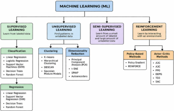
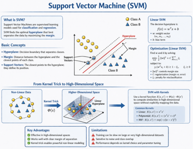
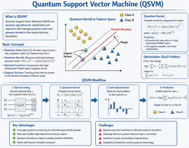
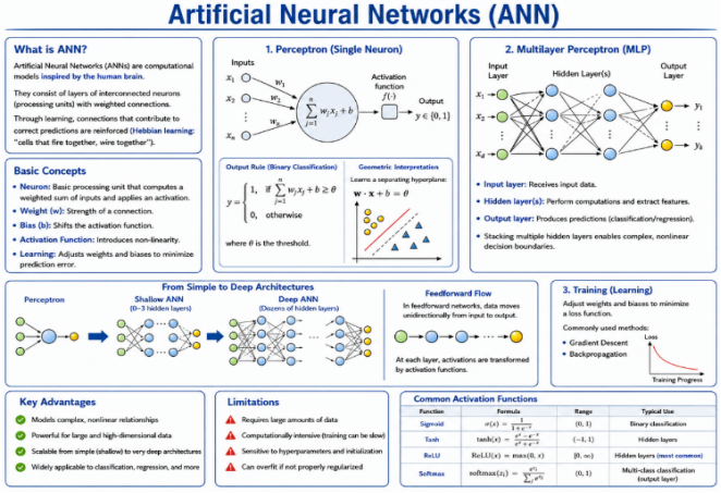
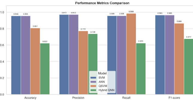
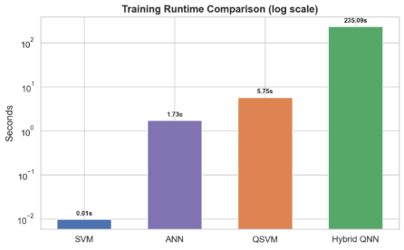
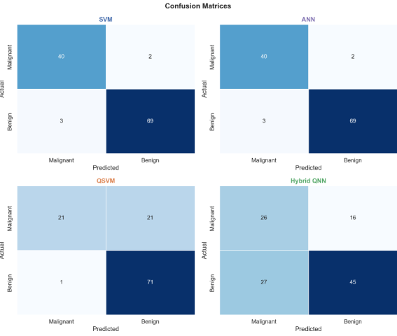
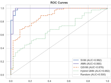
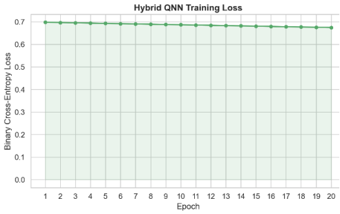
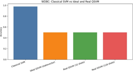




 Share This Article
 Twitter
 Linked In
 Facebook