Magnetic solitons in quasi-one-dimensional anisotropic Heisenberg magnets are stable nonlinear excitations that can transport spin, energy, and information over long distances. This paper develops a practical theory for neutron (inelastic) scattering from such solitons and clarifies how quantum and thermal fluctuations control the observable spectrum. Starting from an easy-axis Heisenberg ferromagnet with nearest-neighbor exchange and uniaxial anisotropy, a single soliton is treated as a particle-like mode characterized by conserved quantities that may be interpreted as the number of magnons bound in the soliton and the soliton quasi-momentum. Exploiting the integrability of the model and the possibility of separating kinetic and potential energies in action-angle variables, the soliton contribution to the dynamic structure factor S(q, ω) and to the double-differential scattering cross section is derived. The derivation adapts the Kawasaki-type approach used in earlier soliton scattering studies, but is reformulated here in a simplified and transparent way that yields a general working formula without cumbersome intermediate steps. The resulting response naturally splits into quasi-elastic and inelastic parts. Soliton translation produces a pronounced quasi-elastic intensity and can generate central-peak behavior through the soliton’s response to external perturbations. Thermal averaging leads to explicit conditions under which the quasi-elastic component reduces to a Gaussian form; the analysis also delineates when this approximation fails, in particular for “massive” solitons with large bound-magnon number. At larger energy transfers, scattering into excited soliton states becomes possible, providing access to internal soliton modes and to dissipation mechanisms in real materials. The obtained expressions connect measurable line shapes and spectral weights to soliton width, effective mass, stability, and transport characteristics. Overall, the work provides a concrete basis for interpreting neutron-scattering signatures of solitonic states in quasi-one-dimensional magnets and for designing experiments that isolate their contribution, with relevance to nonlinear magnetic dynamics, spin-transport phenomena, and prospective quantum-technology applications.
| Published in | American Journal of Modern Physics (Volume 15, Issue 2) |
| DOI | 10.11648/j.ajmp.20261502.15 |
| Page(s) | 43-54 |
| Creative Commons |
This is an Open Access article, distributed under the terms of the Creative Commons Attribution 4.0 International License (http://creativecommons.org/licenses/by/4.0/), which permits unrestricted use, distribution and reproduction in any medium or format, provided the original work is properly cited. |
| Copyright |
Copyright © The Author(s), 2026. Published by Science Publishing Group |
Magnetic Solitons, Anisotropic Heisenberg Magnet, Easy-axis Ferromagnet, Neutron (Inelastic) Scattering
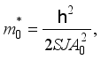
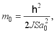
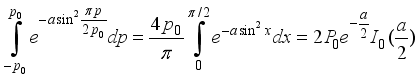
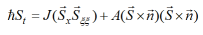 (1)
(1)  (2)
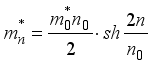
(2) 
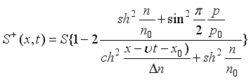
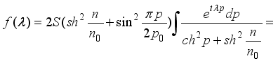
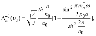
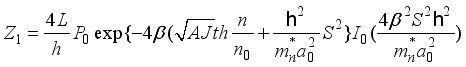
 (3)
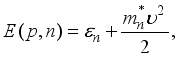
(3) 
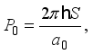
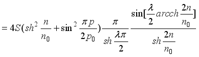
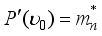
 (4)
(4) 

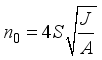
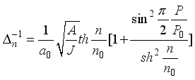
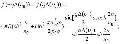
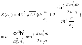
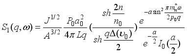
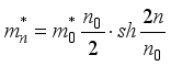 (5)
(5) 
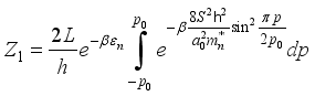
 (6)
(6) 
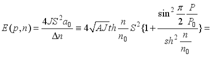
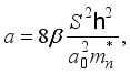
 (7)
(7) 
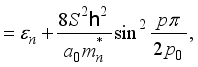
 (8)
(8) 
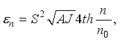
 (9)
(9)  (10)
(10)  (11)
(11)  (12)
(12) | [1] | Makhankov, A. V., Makhankov, V. G. Spin coherent states, Holstein–Primakoff transformations for Heisenberg spin chain models, and status of the Landau–Lifshitz equation. Physica Status Solidi (b), 1987, 145, 669–678. |
| [2] | Mikeska, H.-J., Kolezhuk, A. K. One-dimensional magnetism. In: Schollwöck, U., Richter, J., Farnell, D. J. J., Bishop, R. F. (eds.). Quantum Magnetism. Lecture Notes in Physics, vol. 645. Berlin, Heidelberg: Springer, 2004, pp. 1–83. |
| [3] | Bloch, F. On the theory of ferromagnetism. Zeitschrift für Physik, 1930, 61, 206–219. |
| [4] | Novikov, V. N. Theory and Techniques of Neutron Scattering. St. Petersburg: Polytechnic University Press, 2010. |
| [5] | Balents, L. Spin liquids in frustrated magnets. Nature, 2010, 464, 199–208. |
| [6] | Ivanov, B. A., Kolesnichenko, Yu. A. Magnon solitons in anisotropic ferromagnets. JETP, 1999. |
| [7] | Brockmann, M., et al. Quantum and thermal fluctuations in soliton dynamics in quasi-one-dimensional spin systems. Physical Review B, 2013, 87. |
| [8] | Baryakhtar, V. G., Ivanov, B. A., Chetkin, M. V. Dynamics of Magnetic Solitons. Kyiv: Naukova Dumka, 1983. |
| [9] | Abdulloev, Kh. O., Makhankov, A. V. Quasiclassical behavior of initial spin wave packets within the easy-plane Heisenberg model. Izvestiya of the Academy of Sciences of the Republic of Tajikistan, 1991, III(2), 170–174. |
| [10] | Abdulloev, Kh. O., Muminov, Kh. Kh., Rahimi, F. Coherent states of the SU(4) group in real parametrization and Hamiltonian equations of motion. Reports of the Academy of Sciences of the Republic of Tajikistan, 1993, Nos. 8–9, 20–24. |
| [11] | Abdulloev, Kh. O., Muminov, Kh. Kh., Maksudov, A. On a system of equations in the theory of spin waves. Reports of the Academy of Sciences of the Tajik SSR, 1991, 34(8), 64–68. |
| [12] | Abdulloev, Kh. O., Muminov, Kh. Kh., Maksudov, A. On the correspondence of quantum and classical models in the theory of condensed matter. In: Proceedings of the All-Union Seminar “Interparticle Interactions in Solutions”, 1990, pp. 51–58. |
| [13] | Abdulloev, Kh. O., Rakhimi, F. Exact one-soliton solutions of the dynamic equations of motion of a uniaxial Heisenberg ferromagnet in the SU(3)/SU(2) × U(1) space. Reports of the Academy of Sciences of the Republic of Tajikistan, 40(3–4), 77–80. |
| [14] | Kawasaki, K. Time correlation function of the Sine-Gordon system. Progress of Theoretical Physics, 1976, 55(6), 2029–2030. |
| [15] | Mikeska, H.-J. Solitons in a one-dimensional magnet with an easy plane. Journal of Physics C: Solid State Physics, 1978, 11, L29–L32. |
| [16] | Kjems, J. K., Steiner, M. Evidence for soliton modes in the one-dimensional ferromagnet CsNiF3_33. Physical Review Letters, 1978, 41(16), 1137–1140. |
| [17] | Steiner, M., Kakurai, K., Knop, W., Kjems, J. K. Neutron inelastic scattering study of transverse spin fluctuations in CsNiF3_33: A soliton-only central peak. Solid State Communications, 1982, 41(4), 329–332. |
| [18] | Fedyanin, V. K., Makhankov, V. G. Physica Scripta, 1983, 28, 221–228. |
| [19] | Boothroyd, A. T. Principles of Neutron Scattering from Condensed Matter. Oxford: Oxford University Press, 2020. |
| [20] | Scheie, A., Sherman, N. E., Dupont, M., et al. Detection of Kardar–Parisi–Zhang hydrodynamics in a quantum Heisenberg spin-1/2 chain. Nature Physics, 2021, 17(6), 726–730. |
| [21] | Gopalakrishnan, S., Vasseur, R. Kinetic theory of spin diffusion and superdiffusion in XXZ spin chains. Physical Review Letters, 2019, 122, 127202. |
| [22] | Doyon, B., Gopalakrishnan, S., Møller, F., Schmiedmayer, J., Vasseur, R. Generalized hydrodynamics: A perspective. Physical Review X, 2025, 15(1), 010501. |
| [23] | Shao, H., Sandvik, A. W. Progress on stochastic analytic continuation of quantum Monte Carlo data. Physics Reports, 2023, 1003, 1–88. |
| [24] | Zvyagin, S. Spin dynamics in quantum sine-Gordon spin chains: High-field ESR studies. Applied Magnetic Resonance, 2021, 52, 337–348. |
| [25] | Vaidya, S., Curley, S. P. M., Manuel, P., et al. Magnetic properties of a staggered S = 1 chain with an alternating single-ion anisotropy direction. Physical Review B, 2025, 111, 014421. |
APA Style
Rahimi, F. (2026). Neutron Scattering on Solitons in Anisotropic Magnets: Quantum and Thermal Aspects. American Journal of Modern Physics, 15(2), 43-54. https://doi.org/10.11648/j.ajmp.20261502.15
ACS Style
Rahimi, F. Neutron Scattering on Solitons in Anisotropic Magnets: Quantum and Thermal Aspects. Am. J. Mod. Phys. 2026, 15(2), 43-54. doi: 10.11648/j.ajmp.20261502.15
@article{10.11648/j.ajmp.20261502.15,
  author = {Farhod Rahimi},
  title = {Neutron Scattering on Solitons in Anisotropic Magnets: Quantum and Thermal Aspects},
  journal = {American Journal of Modern Physics},
  volume = {15},
  number = {2},
  pages = {43-54},
  doi = {10.11648/j.ajmp.20261502.15},
  url = {https://doi.org/10.11648/j.ajmp.20261502.15},
  eprint = {https://article.sciencepublishinggroup.com/pdf/10.11648.j.ajmp.20261502.15},
  abstract = {Magnetic solitons in quasi-one-dimensional anisotropic Heisenberg magnets are stable nonlinear excitations that can transport spin, energy, and information over long distances. This paper develops a practical theory for neutron (inelastic) scattering from such solitons and clarifies how quantum and thermal fluctuations control the observable spectrum. Starting from an easy-axis Heisenberg ferromagnet with nearest-neighbor exchange and uniaxial anisotropy, a single soliton is treated as a particle-like mode characterized by conserved quantities that may be interpreted as the number of magnons bound in the soliton and the soliton quasi-momentum. Exploiting the integrability of the model and the possibility of separating kinetic and potential energies in action-angle variables, the soliton contribution to the dynamic structure factor S(q, ω) and to the double-differential scattering cross section is derived. The derivation adapts the Kawasaki-type approach used in earlier soliton scattering studies, but is reformulated here in a simplified and transparent way that yields a general working formula without cumbersome intermediate steps. The resulting response naturally splits into quasi-elastic and inelastic parts. Soliton translation produces a pronounced quasi-elastic intensity and can generate central-peak behavior through the soliton’s response to external perturbations. Thermal averaging leads to explicit conditions under which the quasi-elastic component reduces to a Gaussian form; the analysis also delineates when this approximation fails, in particular for “massive” solitons with large bound-magnon number. At larger energy transfers, scattering into excited soliton states becomes possible, providing access to internal soliton modes and to dissipation mechanisms in real materials. The obtained expressions connect measurable line shapes and spectral weights to soliton width, effective mass, stability, and transport characteristics. Overall, the work provides a concrete basis for interpreting neutron-scattering signatures of solitonic states in quasi-one-dimensional magnets and for designing experiments that isolate their contribution, with relevance to nonlinear magnetic dynamics, spin-transport phenomena, and prospective quantum-technology applications.},
 year = {2026}
}
TY  - JOUR
T1  - Neutron Scattering on Solitons in Anisotropic Magnets: Quantum and Thermal Aspects
AU  - Farhod Rahimi
Y1  - 2026/04/02
PY  - 2026
N1  - https://doi.org/10.11648/j.ajmp.20261502.15
DO  - 10.11648/j.ajmp.20261502.15
T2  - American Journal of Modern Physics
JF  - American Journal of Modern Physics
JO  - American Journal of Modern Physics
SP  - 43
EP  - 54
PB  - Science Publishing Group
SN  - 2326-8891
UR  - https://doi.org/10.11648/j.ajmp.20261502.15
AB  - Magnetic solitons in quasi-one-dimensional anisotropic Heisenberg magnets are stable nonlinear excitations that can transport spin, energy, and information over long distances. This paper develops a practical theory for neutron (inelastic) scattering from such solitons and clarifies how quantum and thermal fluctuations control the observable spectrum. Starting from an easy-axis Heisenberg ferromagnet with nearest-neighbor exchange and uniaxial anisotropy, a single soliton is treated as a particle-like mode characterized by conserved quantities that may be interpreted as the number of magnons bound in the soliton and the soliton quasi-momentum. Exploiting the integrability of the model and the possibility of separating kinetic and potential energies in action-angle variables, the soliton contribution to the dynamic structure factor S(q, ω) and to the double-differential scattering cross section is derived. The derivation adapts the Kawasaki-type approach used in earlier soliton scattering studies, but is reformulated here in a simplified and transparent way that yields a general working formula without cumbersome intermediate steps. The resulting response naturally splits into quasi-elastic and inelastic parts. Soliton translation produces a pronounced quasi-elastic intensity and can generate central-peak behavior through the soliton’s response to external perturbations. Thermal averaging leads to explicit conditions under which the quasi-elastic component reduces to a Gaussian form; the analysis also delineates when this approximation fails, in particular for “massive” solitons with large bound-magnon number. At larger energy transfers, scattering into excited soliton states becomes possible, providing access to internal soliton modes and to dissipation mechanisms in real materials. The obtained expressions connect measurable line shapes and spectral weights to soliton width, effective mass, stability, and transport characteristics. Overall, the work provides a concrete basis for interpreting neutron-scattering signatures of solitonic states in quasi-one-dimensional magnets and for designing experiments that isolate their contribution, with relevance to nonlinear magnetic dynamics, spin-transport phenomena, and prospective quantum-technology applications.
VL  - 15
IS  - 2
ER  -
National Academy of Sciences of Tajikistan, Umarov Physical-Technical Institute, Dushanbe, Tajikistan
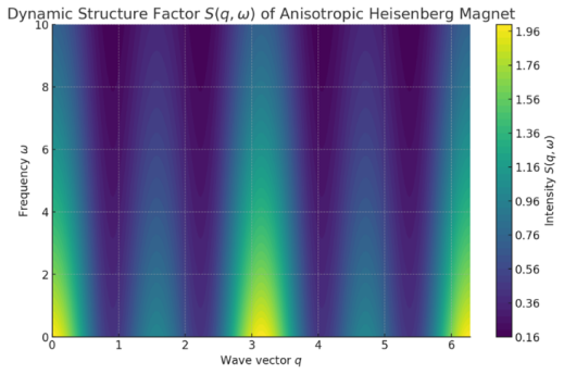
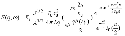
Figure 1. Dynamic structure factor S(,ω) as a function of the wave vector q and frequency ω for an anisotropic Heisenberg magnet.
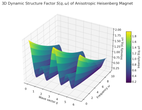
Figure 2. Three-dimensional plot of the dynamic structure factor S(,ω)S as a function of the wave vector q and frequency ω for an anisotropic Heisenberg magnet. The surface height and color represent the intensity of the structure factor.
Figure 3. The dynamic structure factor S(q,ω,T) as a function of the wave vector q, frequency ω, and temperature T, illustrating the influence of temperature on the dynamic properties of the system.
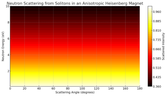
Figure 4. Map of the neutron scattering intensity distribution from soliton states in an anisotropic Heisenberg magnet in the coordinates “scattering angle – scattered neutron energy.” The intensity is represented by a color scale, where darker regions correspond to higher scattering values.
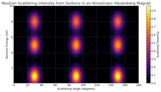
Figure 5. Map of the neutron scattering intensity distribution obtained with consideration of the influence of solitons in an anisotropic Heisenberg magnet. In the coordinates “scattering angle–neutron energy,” resonance peaks are observed, reflecting the characteristic features of solitonic excitations. The color scale indicates the magnitude of the scattering intensity.
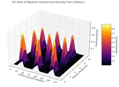
Figure 6. Three-dimensional map of the neutron scattering intensity distribution from soliton states in an anisotropic Heisenberg magnet. In the coordinates “scattering angle–neutron energy,” both the surface height and the color scale characterize the magnitude of the scattering intensity, where darker regions correspond to higher values.
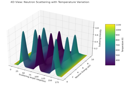
Figure 7. Three-dimensional visualization of the neutron scattering intensity in an anisotropic Heisenberg magnet with the temperature factor taken into account. The surface color scale characterizes the magnitude of the scattering intensity and its variation with temperature, providing a clear representation of the temperature dependence of the process under study.
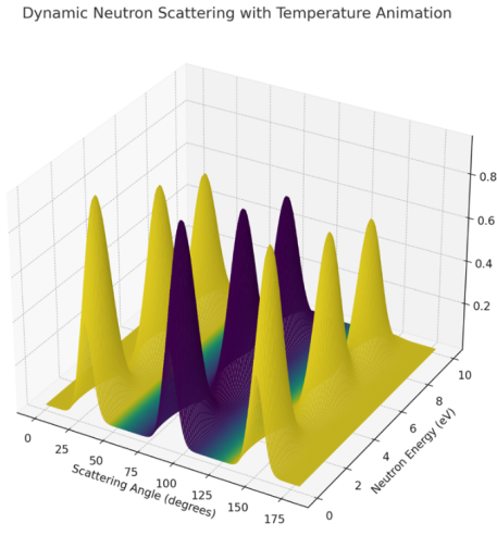
Figure 8. Animated visualization of the temporal evolution of the temperature profile and its effect on the neutron scattering intensity from soliton states in an anisotropic Heisenberg magnet. Variations in temperature are accompanied by corresponding changes in the color distribution of the graph, providing a clear illustration of the influence of the temperature factor on the dynamic processes in the material.
Information