Cross-domain Network Intrusion Detection Based on 1-D CNN, PCA, and GloVe Embedding

Gabriel Babatunde Iwasokun; Ahmed Ojodu; Johnson Adeleke Adeyiga; Oludare Johnson Olaleye; Mojisola Olajumoke Ogunseye; Ibraheem Temitope Jimoh; David Bamidele Adewole

doi:doi:10.11648/j.ajnc.20261502.11

Research Article |

| Peer-Reviewed

Cross-domain Network Intrusion Detection Based on 1-D CNN, PCA, and GloVe Embedding

Gabriel Babatunde Iwasokun^*

, Ahmed Ojodu, Johnson Adeleke Adeyiga

, Oludare Johnson Olaleye, Mojisola Olajumoke Ogunseye

, Ibraheem Temitope Jimoh

, David Bamidele Adewole

Published in American Journal of Networks and Communications (Volume 15, Issue 2)

Received: 29 June 2026 Accepted: 8 July 2026 Published: 28 July 2026

Views: Downloads:

Download PDF

Share This Article

Twitter
Linked In
Facebook

Abstract

The existing communication networks are currently encompassed with various malicious activities that aim to compromise the confidentiality, integrity, and availability of data and systems. The activities include malware, phishing, ransomware, Distributed Denial of Service (DDoS) attacks, and insider attacks. The rapid evolution of these threats necessitates the development of advanced and adaptable intrusion detection systems (IDS) capable of operating across diverse network environments. This paper presents the design of a cross-domain network intrusion detection system that leverages a convolutional neural network and principal components analysis to enhance network intrusion detection accuracy and generalisation. The design integrates GloVe (Global Vectors for Word Representation) embeddings to transform network traffic data into a meaningful feature space, utilises Principal Component Analysis (PCA) for dimensionality reduction, and employs a one-dimensional Convolutional Neural Network (1D-CNN) for efficient classification of network activities. The design also considered preprocessing of multiple intrusion detection data from various network domains, and each data is subjected to GloVe-based feature extraction to generate dense vector representations, which are subsequently concatenated to form a unified embedding layer. The PCA component is required for mitigating the issues with dimensionality and enhancing computational efficiency. It will also be used to extract some significant features before the 1D-CNN-enabled intrusion classification. The experimental study of the system established its practical function and suitability for a very high, accurate, and reliable detection of intrusions in multi-domain networks.

Published in	American Journal of Networks and Communications (Volume 15, Issue 2)
DOI	10.11648/j.ajnc.20261502.11
Page(s)	33-48
Creative Commons	This is an Open Access article, distributed under the terms of the Creative Commons Attribution 4.0 International License (http://creativecommons.org/licenses/by/4.0/), which permits unrestricted use, distribution and reproduction in any medium or format, provided the original work is properly cited.
Copyright	Copyright © The Author(s), 2026. Published by Science Publishing Group

Keywords

Multi-domain, Intrusion Detection, Convolutional Neural Network, Principal Components Analysis, GloVe Embedding

1. Introduction

The growth in modern networks' complexity and interconnectivity has amplified the demand for strong security measures to safeguard sensitive data and critical infrastructure. A Network Intrusion Detection System (NIDS) is indispensable in the detection and prevention of malicious activities within network environments. As organisations experience multi-lateral expansion and integration, the need for cross-domain NIDS that can effectively monitor and analyse network traffic across diverse environments has continued to be on increase

[1]

. A NIDS is a security mechanism for monitoring network traffic to detect suspicious events and likely threats. It examines network packets to know the patterns or anomalies that could signal malicious behaviour like unauthorised access attempts, malware spread, or data exfiltration. Traditional or old-style NIDS rely on pre-defined guidelines and monicker databases to discover branded threats. It also relies on some incongruity recognition systems to identify unfamiliar network behaviour. This class of NIDS is often restricted to certain network domains and may not successfully detect intrusions across multiple domains or heterogeneous network environments. Its trials include the assortment of networks, clambering problems, and missing contextual awareness. A cross-domain NIDS with the capacity for monitoring and scrutinising network traffic across numerous network environments is imperative for addressing these challenges. Such a system would enhance security by establishing an all-inclusive discernibility of potential threats across multiple domains

[2]

Deep learning has changed intrusion detection by automating feature extraction and apprehending high-level abstractions of input data. It is used to convert categorical and high-dimensional data into dense and continuous vector representations. In intrusion detection, deep learning embeddings are used to handle numerous data types and promote learning. Typical deep learning embedding techniques include GloVe, the Bert model, and Word2Vec. The challenges to the adoption of deep learning-based cross-domain intrusion detection systems include the fusion of data from different domains, which often requires concatenation and production rule techniques. The concatenation method integrates feature vectors based on end-to-end addition to form a single, more momentous feature vector. The method is direct and conserves all information from the creative features. Based on the growth of the dimensionality of the feature space, the IDS can assume more complex patterns that are linked with intrusions. Conversely, higher dimensionality can lead to increased computational intricacies and risk of overfitting, especially when engaged with restricted training data. These challenges are often addressed by post-concatenation application of dimensionality reduction techniques such as Principal Component Analysis (PCA) or feature selection algorithms

[3]

. These techniques support the identification of the most relevant features, the reduction of noise, and the improvement of the IDS's efficiency. The product rule method encompasses features via element-wise reproduction of feature vectors, seizing interactions between equivalent features from different domains. The method highlights common features and associations, making it mainly effective for recognising synchronised attacks with comparable shapes across domains. It is used to reduce the dimensionality that is related to concatenation, but demands that the feature vectors are of equal length, which compels the need for preprocessing steps for aligning the features

[4]

A cross-domain environment involves the interaction between different security domains, which may vary regarding trust levels, security policies, and data sensitivity. These domains include combinations of classified and unclassified networks, disparate organisational units, or integrated systems from mergers and partnerships. Traditional IDS cannot effectively monitor and analyse data across these varied domains due to limited scope and inability to handle cross-domain data flows

[5]

. The rise of advanced persistent threats (APTs) and multi-vector cyber-attacks exploits the gaps between security domains. Attackers leverage cross-domain interactions to bypass isolated security measures, making it imperative to have an IDS that operates cohesively across these boundaries

[6]

. A cross-domain intrusion detection system (CDIDS) would address this vulnerability by providing visibility and analysis capabilities that transcend individual domains, thereby enhancing the overall security posture. One of the key technical challenges in developing a Cross-Domain Intrusion Detection System (CDIDS) is the integration of diverse data sources. Different domains may use varied data formats, protocols, and security mechanisms. Fusing this data for analysis requires sophisticated feature extraction techniques. Cross-domain interactions inherently increase the attack surface. A CDIDS must detect intrusions and ensure that the data sharing and analysis mechanisms do not introduce new vulnerabilities. Implementing secure communication channels between domains is critical

[7]

. In response to these problems, this study presents the design of a cross-domain intrusion detection platform based on Glove embedding, principal component analysis (PCA), and 1D-CNN. The platform will integrate data sources and network domains to address the challenges of varied data formats and protocols based on effective feature extraction techniques, production rules, and concatenation-induced multi-domain data fusion. The platform will be useful for addressing the complexities of modern network environments, where boundaries between domains are often blurred. This is particularly pertinent in organisations that operate hybrid infrastructures combining on-premises, cloud, and mobile environments. The platform will offer IDS solutions with improved detection of advanced persistent threats (APTs) and multi-vector attacks, as well as create situational awareness by correlating data from diverse sources, which enables more accurate identification of anomalies indicative of malicious activities.

2. Related Works

Intrusion Detection Systems (IDS) can be broadly classified into two main categories: network-based IDS (NIDS) and host-based IDS (HIDS). NIDS monitors network traffic for malicious activities or policy violations, while HIDS focuses on detecting intrusions on individual systems or hosts

[8]

. However, it is worth noting that some sources also mention a third category called specification-based IDS, which is considered particularly suitable for cyber-physical systems like smart grids. NIDS is deployed at key locations within the network to monitor in real-time traffic to and from all connected devices. Host-based intrusion Detection Systems are deployed on individual hosts or devices to monitor incoming and outgoing packets specific to the device. They alert users or administrators to suspicious activity and effectively detect internal intrusions and unauthorised actions

[8, 9]

. Yu et al.

[10]

introduced a Cross-Domain Intrusion Detection Method Based on Nonlinear Augmented Explicit Features (NAEF) to improve the clarity of cross-domain models. The method could enhance the feature space by combining shared, source-domain-specific, and target-domain-specific features. The nonlinear mapping relationship from shared features to unique features in the source and target domains was separately modelled, while the original features in the source and target domains were mapped to uniform explicit features in the augmented space by migration of the nonlinear mapping relationship. With this method, secured communication requires a CDS to match incoming response packets with outgoing requests, which could pose a significant setback. Choi et al.

[11]

introduced a next-generation CDS model to perform stateful correlation between outgoing and incoming application-layer packets. The model could extract user-specified state variables from outgoing traffic and assess incoming packets using predefined rule sets. A prototype-based study of the model established its filtering accuracy over conventional CDS, though with increased processing delay. Layeghy and Portmann

[12]

explored the cross-domain performance of ML-based NIDSs based on an expansive evaluation of some supervised and unsupervised learning models on some of the recently published benchmark NIDS datasets. The evaluation established that none of the models consistently generalises across all datasets, in addition to a significant asymmetry in cross-domain performance. Swapping the source and target domains can lead to substantial variations in classification accuracy. The superiority of unsupervised learning methods over supervised models in the examined scenarios was also confirmed. Layeghy et al.

[13]

carried out the extraction of domain-invariant features using a trained domain adversarial neural network on labelled source domains to extract and utilise a One-Class Support Vector Machine (OSVM) model for network anomaly detection. During testing, the unlabeled data was passed through the feature extractor network to map it into a domain-invariant space, after which OSVM was applied to the extracted features to identify intrusions. Extensive experiments on the NIDS benchmark datasets NFv2-CIC-2018 and NFv2-UNSW-NB15 demonstrated that the model outperformed some other models in cross-domain intrusion detection. Its vulnerability to cyberattacks due to weaknesses in information and communication technologies was also noted.

Zhang et al.

[14]

leveraged transfer learning and public datasets with known attack instances to develop a predictive model for network intrusion detection. The model focuses on mitigating the heterogeneity between datasets by mapping them into a shared latent space and optimising the problem to minimise the distributional differences. A multi-layer perceptron (MLP) classifier was used to transform data and identify attack instances within internal networks. A transfer learning experiment using the NSL-KDD and UNSW-NB15 datasets showed a high cross-domain attack detection accuracy, particularly in DoS to DoS and R2L to exploits scenarios. Abdallah et al.

[15]

presented an IoT and machine learning model to detect deviations from normal network traffic behaviour. Its experimental study established its strong potential for detecting network threats as well as its scalability and cross-domain limitations issues. Zhang et al.

[16]

introduced a federated learning-based IDS to address the problems associated with diverse operational network environments. The framework could preserve the privacy of data, but with high computational demands that pose significant constraints for resource-limited IoT devices, limiting its deployment in the real world.

3. Proposed Platform

The proposed cross-domain intrusion detection model is conceptualized in Figure 1 with stages for preprocessing, GloVe embedding, concatenation of embedding layers, PCA-based dimensionality reduction, 1-dimensional CNN, and intrusion detection. The preprocessing layer oversees the process of data consistency and quality. The GloVe embedding phase of each domain is used to generate domain-specific feature representations that are subsequently concatenated and presented for PCA-based dimensionality reduction for the retention of solely the most relevant features. The final stage of a 1D-CNN is employed for training and prediction that support effective intrusion detection across the various domains.

3.1. 1D-CNN Model

The CNN model is presented in Figure 2 and designed to extract hierarchical patterns from sequential network traffic data and consists of the input, convolutional, pooling, and fully connected layers. While the input layer accepts pre-processed network flow data in a sequential format, the convolutional layer extracts local patterns from the network traffic sequences. The pooling layer is used to reduce the dimensionality and computational complexities, while the fully connected layer is required for the aggregation of the extracted features and for performing final classification.

Download: Download full-size image

Figure 1. Proposed Model Architecture and Components.

Download: Download full-size image

Figure 2. Proposed 1D-CNN Model Architecture and Component.

3.2. Input Layers

The input layers accept pre-processed network flow data and process network traffic as sequential data with shape (

T

F

T

represents the sequence length (number of time steps per traffic flow) and

F

is the number of selected features per time step. The input data is represented as:

X \in R^{T \times F}

(1)

X = [X_{1}, X_{2}, \dots, X_{T}]

is a sequence of feature vectors and

R

is the set of real numbers which show that all elements in

X

are real numbers.

3.3. Data Preprocessing

The multi-domain intrusion dataset must be preprocessed before machine learning techniques are applied to guarantee data consistency, eliminate redundancies, and improve model performance. The following preprocessing procedures are required:

Data Cleaning

Due to packet loss or logging inconsistencies, the raw dataset may contain missing values, duplicate records, or undefined entries. To improve data quality, missing and duplicate values should be dealt with either by the imputation method or by removal. Instances with infinite or undefined values should also be replaced with appropriate defaults or eliminated.

Data Normalization and Standardization

Network traffic data features exhibit diverse numerical ranges, necessitating transformation to improve model interpretability and performance. By normalisation, features will be scaled within a fixed range using the Min-Max scaling formula

[1]

X^{'} = \frac{X - X_{\min}}{X_{\max} - X_{\min}}

(2)

X

is the original value,

X_{\min}

is the minimum value in the dataset, and

X_{\max}

is the maximum value in the dataset. With standardisation, Equation (3) is used to transform the mean and standard deviation of the features to 0 and 1, respectively.

X^{'} = \frac{X - μ}{σ}

(3)

X is the initial value, 𝜇 represents the mean, and 𝜎 is the standard deviation.

3.4. First Convolution Layer

This layer applies 1-D convolutions to the input sequence data based on 32 convolutional filters (kernels). Each of the filters has a size of 3, meaning it slides over 3-time steps at every sequence, and will be used to learn and detect different patterns in the input sequence. The filters also allow the local patterns to be captured across three consecutive steps in the network traffic sequence. The Rectified Linear Unit (ReLU) activation function is applied element-wise after the convolution operation as follows

[17-19]

ReLU (x) = \max (0, x)

(4)

Equation (4) introduces non-linearity and assists the network in learning more complex patterns. The convolution is based on the following:

y_{i, j} = σ (\sum_{k = 0}^{K - 1} X_{i + k, j} W_{k, j} + b_{j})

(5)

y_{i, j}

is the activation at the position,

i,

for filter

j

k

is the kernel size (3 in this case),

W

represents the kernel weights,

b

is the bias term, and

σ (x) = \max (0, x)

is the ReLU activation function, preventing vanishing gradients. The CNN layer extracts local temporal patterns from the input network traffic sequence, while the 32 filters allow the learning of diverse features. The small kernel of size 3 focuses on short-term dependencies, while the ReLU activation is responsible for the acquisition of nonlinear relationships in the data.

First Max Pooling Layer

The first max pooling 1-D layer slides a window of size two across the input, moving by two steps at every move. For each window position, the maximum value within the window is selected as the element in the output feature map. The max pooling is defined as follows

[18-22]

y_{i} = ma x {x_{2 i}, x_{2 i + 1}}

(6)

y_{i}

is the pooled output and

x_{2 i}, x_{2 i + 1}

are the input values within the pooling window.

Second Convolution Layer

This layer uses 64 convolutional filters (twice the number in the first layer) to allow the network to learn more complex patterns. The kernel size of 3 is required to maintain consistency in capturing local patterns across 3-time steps, while the ReLU activation function is required to introduce non-linearity. Specifically, the layer is responsible for the extraction of deeper, more abstract features from the patterns detected by the first layer and the recognition of very complex attack signatures in the network traffic data. The layer is equally responsible for maintaining spatial relationships in the data through the use of local convolutions.

Second Max Pooling Layer

The second max pooling layer in the CNN architecture plays several critical functions that contribute to the model's effectiveness and efficiency. It reduces dimensionality by halving the spatial dimensions of feature maps, thereby decreasing the parameter count and computational requirements. Through feature selection, the layer identifies the most salient information while discarding less significant data, which enhances the model's robustness to minor input translations, mitigates overfitting, and increases the receptive field of subsequent neurons. The max pooling layer also facilitates hierarchical feature learning and noise reduction by selecting the most potent activations, which play a crucial role in balancing feature extraction, reducing computational complexities, and raising efficiency.

Third Convolution Layer

This layer enhances the detection of more complex attack patterns in the network traffic sequences based on 64 convolutional filters that give room for the network to learn increasingly abstract and sophisticated patterns. The kernel size three constantly captures local temporal relationships across the three consecutive time steps, while the ReLU activation function introduces non-linearity, enabling the model to capture complex non-linear patterns in the data. The introduction of the third convolution layer increases the model's capacity to recognise intricate attack signatures and distinguish between normal and malicious network behaviours across different domains.

Embedding Layer

The embedding layer is required for the conversion of the multi-dimensional output of the convolutional layers into a one-dimensional vector. The conversion preceded the passing of data into fully connected (dense) layers for classification or regression tasks. The layer is also responsible for seamless processing and data structuring using dense layers of the one-dimensional input. Based on the input tensor with dimensions

M \times N

. The Flatten operation output is derived from:

X_{flat} \in R^{M \cdot N}

(7)

The Fully Connected Layer of the CNN architecture comprises 64 neurons with ReLU activation. This dense layer performs a linear transformation followed by a non-linear activation function, which enables the extraction of high-level features from the embedded output as follows:

Y = σ (WX + b)

(8)

W

is the weight matrix,

X

is the input vector,

b

is the bias term, and

σ (x) = \max (0, x)

is ReLU activation. The 64 neurons promote the learning of a rich set of features, while the ReLU activation introduces non-linearity to capture complex patterns in the network traffic data. The connected layer is crucial in aggregating spatial and temporal patterns detected by earlier layers to enable effective intrusion detection across different network domains.

3.5. Principal Component Analysis (PCA)

PCA involves data standardisation, computation of covariance, eigenvalues and eigenvectors, selection of top principal components, and data transformation.

Standardisation of Input Data

Let

X

be the input dataset with

n

samples and

d

features

= {x_{1}, x_{2}, \dots, x_{n}

x_{i} \in R^{d}, i = 1, 2, \dots, n

, each feature

j

is standardised using z-score normalisation as follows:

X_{ij}^{*} = \frac{X_{ij} - μ_{j}}{σ_{j}}

(9)

μ_{j}

is the mean of the feature

j

σ_{j}

is the standard deviation of the feature

j

, and

X_{ij}^{*}

is the standardised value of the sample

i

for feature

j

. All the features have a zero mean and unit variance.

Computing the Covariance Matrix

The covariance matrix is derived as follows:

Σ = \frac{1}{n} \sum_{i = 1}^{n} (X_{i} - μ) {(X_{i} - μ)}^{T}

(10)

X_{i}

is the feature vector of the

it h

sample,

μ

is the mean feature vector,

n

is the number of samples,

(X_{i} - μ)

is a column vector of size

d \times 1

and

{(X_{i} - μ)}^{T}

is a row vector of size

1 \times d

. The product

(X_{i} - μ) {(X_{i} - μ)}^{T}

results in

d \times d

matrix, R (the set of real numbers) describes the type of values in the matrix, and

Σ \in R^{d \times d}

is the covariance matrix. Each element

σ_{ij} in Σ

represents the covariance between features

i

and

j

σ_{ij} = \frac{1}{n} \sum_{k = 1}^{n} (X_{ki} - μ_{i}) (X_{kj} - μ_{j})

(11)

A high value of

σ_{ij}

indicates a strong correlation between features

i

and

j

Eigenvalue Decomposition of Covariance Matrix

The covariance matrix is decomposed based on Equation (12).

Σv = λv

(12)

v

is an eigenvector (principal component) and

λ

is the corresponding eigenvalue, which represents the variance explained by the component.

Selecting the Top

k

Principal Components

The number of principal components to retain is based on the explained variance ratio β derived thus:

β = \frac{\sum_{i = 1}^{k} λ_{i}}{\sum_{i = 1}^{d} λ_{i}}

(13)

k

is the number of selected components and

d

is the original number of features. The aim is to select

k

components that retain most of the variance while significantly reducing dimensionality.

Transforming the Data into the New Feature Space

The original dataset

X

is projected onto the new basis using the selected principal components:

X_{r} = X V_{k}

(14)

X_{r}

is the transformed dataset in the reduced feature space, and

V_{k}

is the matrix of the top

k

eigenvectors. This transformation maps high-dimensional network traffic data to a lower-dimensional space.

3.6. Output Layer

The output layer of the proposed architecture has a single neuron with a sigmoid activation function designed for binary classification and prediction of network intrusions. The activation function shown in Equation (15) is used to generate a probability score that represents the likelihood of an instance belonging to a specific class.

σ (x) = \frac{1}{1 + e^{- x}}

(15)

σ (x)

is the attack probability or the likelihood of an intrusion and is in the range

[18]

Loss Function

The loss function is the binary cross-entropy loss and is derived from:

L = - \frac{1}{N} \sum_{i = 1}^{N} [y_{i} lo g (\hat{y_{i}}) + (1 - y_{i}) lo g (1 - \hat{y_{i}})]

(16)

y_{i}

is the actual class label,

\hat{y_{i}}

is the predicted probability and

N

is the number of samples.

Optimization Algorithm

The optimisation algorithm is used to update the model weights and is based on the Adam optimiser

θ_{t + 1}

derived as follows:

θ_{t + 1} = θ_{t} - \frac{α \hat{m_{t}}}{\sqrt{\hat{v_{t}}} + ϵ}

(17)

α

is the learning rate,

\hat{m_{t}} and \hat{v_{t}}

are moment estimates and

ϵ

is the division by zero tolerance index.

The Adam algorithm calculates the exponential stirring average of the slope (first moment) and the squared slope (second moment) of the weights, where the constraints regulate the flattening rates of the stirring averages

[7]

4. Implementation Technique

The implementation of the proposed model was carried out on an HP laptop with 8G RAM and 1 TB HDD on an Intel processor. The software requirements include the Windows operating system, Visual Studio Code IDE, Python programming language, and Streamlit. The Windows operating system provides the required support to other software tools for implementation. It offers a dependable and intuitive environment for executing real-time intrusion detection apps, data preparation libraries, and machine learning frameworks. While Visual Studio Code IDE formed the primary development environment due to its lightweight nature, extensive extension support, and powerful debugging features, Python programming inspired Visual Studio (VS) Code served as the basis for the implementation of the machine learning models. VS Code also provides a virtual environment that offers an optimised development experience with its Jupyter Notebook integration and Python-specific debugging tools. StreamLit is necessary for building an interactive and real-time visualisation interface for network intrusion detection and easy deployment of machine learning models with minimal code.

4.1. Implementation Data

The cross-domain datasets UNSW-NB15, CICIDS2017, and CSE-CIC-IDS2018 were used to train and assess the intrusion detection system. The UNSW-NB15 dataset was assembled by the Australian Centre for Cyber Security in 2015 and comprises about 2.5 million records with 49 distinct attributes. It is made up of simulated DoS, exploits, backdoors, and other regular network traffic attacks. CICIDS2017 was formulated by the Canadian Institute for Cybersecurity and contains 3,119,345 records of network activities. It contains time-stamped events and attacks such as DDoS, Brute Force, and Web Attacks, and is useful for training machine learning models with its over 80 flow features. The CSE-CIC-IDS2018 dataset contains network traffic data from over 50 distinct devices with over 3 million assault records and 13 million benign entries, which makes it ideal for creating systems that can identify intricate threats in various network types. Preprocessed Comma-Separated Value (CSV) files of the extracted flow-based features of the datasets were utilised. The compressed files contain 9.8 million network flows and roughly 80 attributes from which the most relevant ones were selected to create balanced training and testing sets for the investigations. The choice of the UNSW-NB15, CICIDS2017, and CSE-CIC-IDS2018 datasets for the study is premised on their broad spectrum of the prevailing multi-domain network threats.

4.2. Implementation Technique

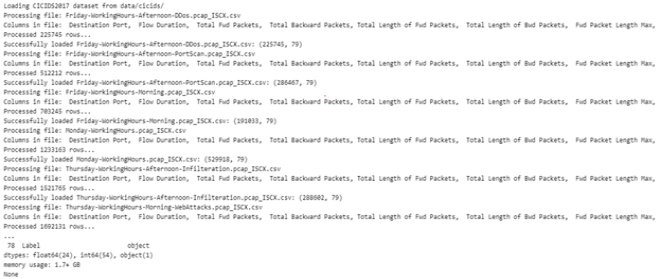
A variety of cutting-edge techniques in a thorough pipeline were used to detect network intrusions. First, the preprocessing and data loading stage lays the groundwork. The large CSV files were effectively handled with a custom load_datasets function, which processed them in pieces, as shown in Figure 3. When working with the large UNSW-NB15, CICIDS2017, and CSE-CIC-IDS2018 datasets, good memory management is promoted through continuous progress updates and firm error handling.

Download: Download full-size image

Figure 3. Screenshot of Data Loading and Initial Processing.

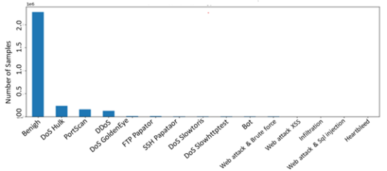
The preprocessing stage is extensively implemented through the preprocess_data function. It is based on the removal of unnecessary network-specific columns like timestamps and IP addresses, management of missing and infinite values through mean imputation, and conversion of categorical features to numeric representations using label encoding. It also involved the standardisation of numerical features to ensure a consistent scale across all variables. The attack distribution for CICIDS2017 is shown in Figure 4.

Download: Download full-size image

Figure 4. Preprocessed data and attack distributions.

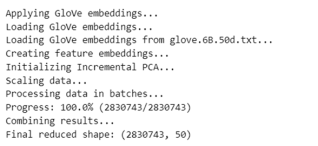
For embedding layer implementation, GloVe (Global Vectors for Word Representation) embeddings were used to create rich feature representations through several coordinated functions. The load_glove_embeddings function was used to retrieve pre-trained word vectors (shown in Figure 5). The create_feature_embeddings function maps feature names to the vectors, handling multi-word features by averaging their component word embeddings. The glove_embedding_layer was used to implement a memory-efficient approach that processed data in manageable batches, created embedded representations of features, and applied incremental PCA to reduce dimensionality while preserving important patterns. The dimensionality reduction through PCA was carefully implemented to handle large datasets, allowing the processing of data in batches without total memory loading.

Download: Download full-size image

Figure 5. Screenshot of GloVe embedding and PCA process.

A 1D-CNN is the fundamental component of the detection system. Higher-level features were gradually extracted from the input data, with each convolutional layer picking up increasingly intricate patterns. The system includes comprehensive evaluation and visualisation capabilities and generates detailed visualisations of the PCA analysis results, training metrics over time, including accuracy and loss curves, a confusion matrix to assess detection performance, and the key performance metrics (accuracy, precision, recall, F1 score). Finally, the implementation was based on the save_model_components function that created timestamped directories containing the trained CNN model, fitted IPCA model, and feature names and configurations. The combination of GloVe embeddings and CNN architecture represents an innovative approach to network intrusion detection, leveraging a semantic understanding of features and robust pattern recognition capabilities.

The training process was set up with a batch size of 32 to balance training speed and memory usage, a validation split of 0.2 to set aside 20% of the training data for validation during the training process, and 10 epochs to allow for enough learning iterations while avoiding overfitting. The other parameters are presented in Table 1.

Table 1. 1D-CNN training parameters.

Hyperparameter	Value
1D-CNN Layers	3
Max Pooling	2
Kernel Size	3
Activation (Dense Layer 1)	ReLU
Activation (Dense Layer 2)	Sigmoid
Optimizer	Adam
Loss Function	Binary Crossentropy
Metrics	Accuracy
Epochs	10
Batch Size	32
Validation Split	0.2
Verbose	1

The experimental evaluation of the 1D-CNN-based Network Intrusion Detection System was carried out as a Streamlit web application, which offers an intuitive drag-and-drop interface for uploading and analysing network traffic data. The application also supported real-time processing and visualisation of network traffic analysis. A pre-trained CNN model was integrated with an efficient data processing pipeline for practical deployment scenarios. The raw dataset features included the basic flow metrics (duration, packet counts), packet length statistics (forward/backward), protocol-specific indicators, and traffic pattern identifiers. A sophisticated preprocessing pipeline that transforms raw network data into model-ready format was implemented. The initial data processing involved a raw feature count of 77 dimensions and a sample size of 225,745 network flows. The dimensionality reduction involved the implementation of Incremental Principal Component Analysis (IPCA), reduction to 50 optimal features, preservation of critical network flow characteristics, and final data shape normalisation (225745, 50, 1).

4.3. Result Discussion

The attack scenarios of the datasets from multiple domains, UNSW-NB15, CICIDS2017, and CSE-CIC-IDS2018, without prior training on these datasets, are presented in Table 2. The datasets were subjected to preprocessing to standardise features and eliminate inconsistencies, ensuring effective integration for intrusion detection. After preprocessing, GloVe converted the data into a feature representation and encoded the network traffic attributes into dense vector representations to improve the model's capacity to identify anomalies in network traffic and generalise various datasets. The model learnt from several datasets at once, thanks to the embeddings into a concatenated embedding layer, which reduced domain-specific biases while improving generalisation across network contexts. The most important attributes were extracted, and feature redundancy was decreased using PCA.

By lowering dimensionality while maintaining crucial data variations, PCA increased computing efficiency by ensuring that only the most pertinent features were presented to the classifier. The 1D-CNN performed well with sequential data such as network traffic records and processed the refined feature set. The CNN successfully recognised intricate attack patterns by capturing spatial relationships in network traffic. The CNN's numerous layers allowed the identification of anomalous sequences and temporal correlations in packet flows. Consequently, the model can forecast certain incursions.

Table 2. Attack scenarios before and after model training.

Attack Type	Dataset	Actual	Before	After
DDoS	UNSW-NB15	8,027	1,294	2,214
	CICIDS2017	8,027	1,983	3,456
	CSE-CIC-IDS2018	8,027	3,152	5,342
PortScan	UNSW-NB15	15,034	2,942	5,274
	CICIDS2017	15,034	4,295	7,217
	CSE-CIC-IDS2018	15,034	5,754	10,430
Infiltration	UNSW-NB15	4,332	647	926
	CICIDS2017	4,332	1,239	1,987
	CSE-CIC-IDS2018	4,332	1,398	2,495
WebAttacks	UNSW-NB15	14,875	2,858	4,930
	CICIDS2017	14,875	4,967	7,840
	CSE-CIC-IDS2018	14,875	5,902	9,677

The number of attack instances across all datasets for the DDoS attack was 8,027. Prior to training, the detection rates were relatively low, with only 1,294 (16.1%) detected in UNSW-NB15, 1,983 (24.7%) in CICIDS2017, and 3,152 (39.3%) in CSE-CIC-IDS2018. The post-training detection rates of 2,214 (27.6%), 3,456 (43.1%), and 5,342 (66.6%), respectively, showed improvements in detection accuracy, with an average increase of approximately 67.4% across the three datasets. Similarly, for the PortScan attack, the model initially identified 2,942 (19.6%) attacks in UNSW-NB15, 4,295 (28.6%) in CICIDS2017, and 5,754 (38.3%) in CSE-CIC-IDS2018. Post-training, detection rates increased to 5,274 (35.1%), 7,217 (48.0%), and 10,430 (69.4%), respectively, indicating an overall improvement of about 73.4%. For the Infiltration attack, before training, the detection rates were lower, with only 647 (14.9%) identified in UNSW-NB15, 1,239 (28.6%) in CICIDS2017, and 1,398 (32.3%) in CSE-CIC-IDS2018. After model training, these values improved to 926 (21.4%), 1,987 (45.9%), and 2,495 (57.6%), showing a significant enhancement in detection performance, with an average improvement of 88.5%. Finally, for Web attacks, the pre-training detection rates were 2,858 (19.2%) in UNSW-NB15, 4,967 (33.4%) in CICIDS2017, and 5,902 (39.7%) in CSE-CIC-IDS2018. Following training, detection increased to 4,930 (33.1%), 7,840 (52.7%), and 9,677 (65.0%), respectively, leading to an overall increase of approximately 67.3%. These results established that the proposed model significantly enhances attack detection accuracy across multiple datasets. The highest improvement was observed in Infiltration attacks (88.5%), while other attack types also showed substantial increases, indicating the robustness of the model in recognising diverse cyber threats. This improvement suggests that incorporating advanced detection techniques, such as feature selection and anomaly detection, can significantly enhance cybersecurity in real-time mode.

4.4. Model Evaluation

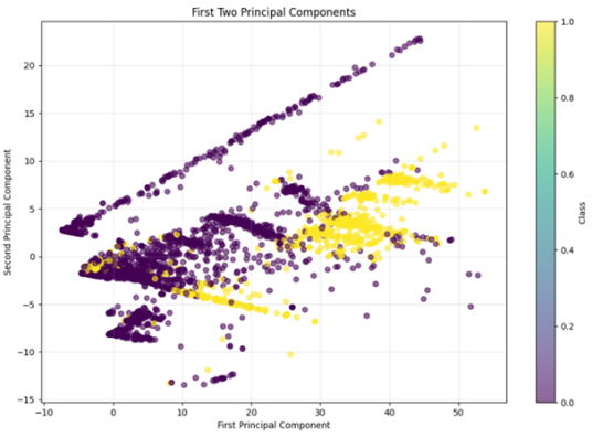
The Principal Components scatter plot shown in Figure 6 provides crucial insights into the structure of the UNSW-NB15, CICIDS2017, and CSE-CIC-IDS2018 network traffic datasets. Each point represents a network flow, with the x and y axes showing the first and second principal components. The distinct colouring scheme (purple and yellow) separates regular traffic (yellow) from various cyber-attacks (purple), demonstrating how PCA can help distinguish between benign and malicious network behaviour. The diagonal line pattern visible in the upper portion of the plot suggests a strong linear relationship between certain attack types, possibly indicating similarities in their network signatures. The spread of points, particularly in the range of -10 to 50 on the first component and -15 to 25 on the second component, reveals the high dimensionality of network traffic features being effectively compressed into two dimensions while preserving meaningful separation between traffic classes.

Download: Download full-size image

Figure 6. The Scatter plot of PCA.

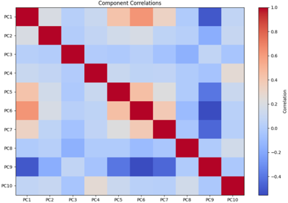
The component correlations heatmap shown in Figure 7 reveals the relationships between the first ten principal components of the transformed UNSW-NB15, CICIDS2017, and CSE-CIC-IDS2018 features. The diagonal red squares represent the perfect self-correlation of each component, while the varying shades of blue and red in off-diagonal elements show the correlations between different components. Of particular interest are the moderate correlations between PC1 and PC5-PC7 (shown in light red), which might indicate that these components capture related aspects of network behaviour, such as different characteristics of similar attack patterns. The predominantly light blue colouring in many off-diagonal elements suggests slight negative correlations between components, which could represent trade-offs between different aspects of network traffic patterns. This visualisation is valuable for understanding how different transformed features relate to each other in the context of network traffic analysis.

Download: Download full-size image

Figure 7. Component Correlations heatmap.

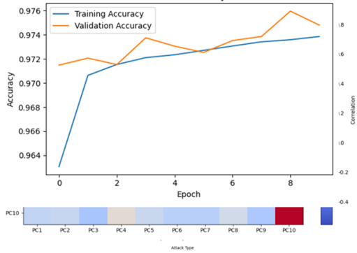
The training and validation performance of a machine learning model trained on the UNSW-NB15, CICIDS2017, and CSE-CIC-IDS2018 network intrusion detection dataset over several epochs is depicted in the model accuracy graph shown in Figure 8. During the first two epochs, the training accuracy (blue line) exhibits a distinctive rapid improvement, rising from roughly 96.3% to 97.0% shortly before gradually increasing. This initial notable enhancement indicates that the model rapidly picks up the fundamental patterns that differentiate between typical network traffic and different types of cyberattacks within the dataset. The validation accuracy (orange line), which peaks at epoch eight at about 97.6%, is more variable and begins higher at about 97.1%. The validation accuracy is consistently above or near the training accuracy, which is odd and indicates that the model may be generalising particularly well to new network traffic patterns. This could be because of the intrinsic structure of network attack patterns in the three datasets, or it could be the result of good feature engineering.

Download: Download full-size image

Figure 8. Model training and validation performance accuracy.

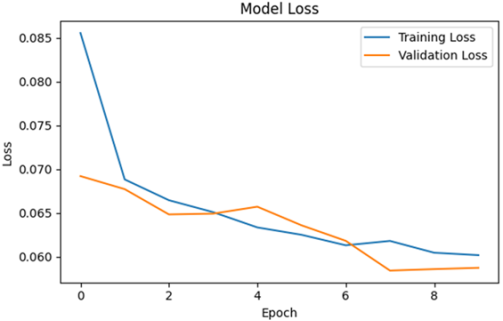
Upon closer inspection of the Model Accuracy graph, both curves exhibit a generally positive trend, but after the first few epochs, the returns start to decline. Although this trend is common in machine learning models, network intrusion detection is critical. The model's high accuracy values (above 96%) show that it can effectively differentiate between malicious and legitimate network traffic, essential for real-world implementation in network security systems. The model may be beginning to identify more subtle patterns in the attack signatures found in the UNSW-NB15, CICIDS2017, and CSE-CIC-IDS2018 datasets, as evidenced by the modest disagreement between training and validation accuracy towards the later epochs (6-9). Instead of overfitting to training data noise, the validation accuracy's continued strength indicates that these patterns characterise actual characteristics of the various assault types. The Model Loss graph in Figure 9 offers complementary information regarding the learning process, which illustrates how the error rates for the training (blue line) and validation (orange line) sets decline over time. The training loss begins noticeably greater at about 8.5% and decreases sharply in the first period before gradually declining. The model's initial learning of the most distinguishing characteristics that define various types of network traffic in the three datasets is represented by this quick initial decrease in loss, which is correlated with the quick improvement in accuracy seen in the first few epochs. The smooth, consistent decrease in both loss curves suggests that the model is learning stably. This is particularly important for network security applications where reliability and consistency are crucial.

The validation loss curve in the Model Loss graph follows a similar downward trend but with some interesting characteristics. It starts lower than the training loss at around 6.9% and generally maintains a smoother descent than the training loss. The convergence of both loss curves around epoch 4, followed by their continued close tracking, indicates the model's generalisation capabilities. The final loss values of approximately 6% for both curves suggest that the model has reached a stable state where it can reliably classify network traffic across both seen and unseen examples from the UNSW-NB15, CICIDS2017, and CSE-CIC-IDS2018 datasets. This behaviour is particularly desirable in intrusion detection systems, as it indicates that the model has learned robust features that characterise different types of network behaviour without becoming overly specialised in the training data.

Download: Download full-size image

Figure 9. Model Loss.

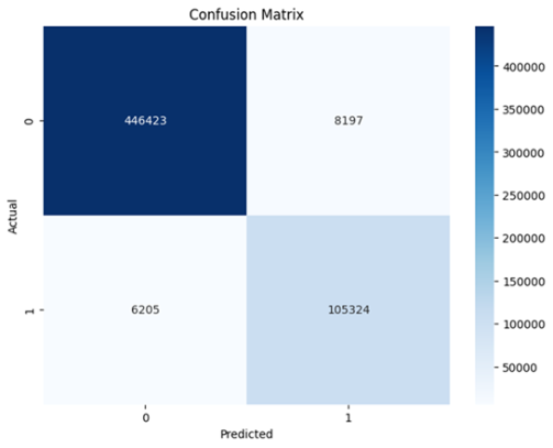
The confusion matrix presented in Figure 10 provides a comprehensive overview of the model's classification performance for the three datasets for intrusion detection. The quadrants of the matrix divide the model's predictions into four main groups. 446,423 true negatives or typical network traffic accurately classified as benign are in the top-left quadrant. This significant frequency of true negatives is essential for a network intrusion detection system since it shows that the model is very good at identifying typical traffic patterns and avoiding false alarms, which could otherwise overwhelm security analysts with false alarms.

Download: Download full-size image

Figure 10. Confusion Matrix.

The 105,324 true positives in the bottom-right quadrant indicate malicious traffic that was accurately classified as an attack. This high value indicates that the model can identify different network attacks in the UNSW-NB15, CICIDS2017, and CSE-CIC-IDS2018 datasets. These attack scenarios include brute force, DDoS, web attacks, and infiltration efforts. Recognising this large number of attack instances accurately is helpful because they constitute the security dangers that must be detected and dealt with in a real-world network setup. The model's error patterns are seen in the off-diagonal elements. 8,197 false positives, or instances when benign traffic was mistakenly identified as malicious, are displayed in the top-right quadrant. In a real-world scenario, each false positive is an unwarranted security warning that might divert security personnel from grave dangers, even though this number is minor compared to the true negatives (representing only roughly 1.8% of all regular traffic). Nonetheless, considering the delicate nature of network security, a small portion of false positives is sometimes regarded as a reasonable trade-off to guarantee high detection rates of actual assaults.

The bottom-left quadrant displays 6,205 false negatives, where actual attacks were misclassified as regular traffic. This number, while relatively small compared to the true positives (about 5.6% of actual attacks), represents perhaps the most critical type of error in an intrusion detection context, as each false negative represents a security threat that would go undetected. The fact that this number is lower than the false positives suggests that the model is appropriately tuned for security applications, where missing an attack (false negative) is generally considered more serious than raising a false alarm (false positive). To provide additional context from the UNSW-NB15, CICIDS2017, and CSE-CIC-IDS2018 datasets, these missed attacks could include more subtle or sophisticated attack patterns that share characteristics with regular traffic, such as low-and-slow attacks or carefully crafted infiltration attempts. Given these numbers, the important metrics can be calculated for this model's performance on the UNSW-NB15, CICIDS2017, and CSE-CIC-IDS2018 datasets. The overall accuracy is approximately 90.91%, which aligns with the high accuracy values observed in the previous training graphs. The model achieves a precision of approximately 89% for attack detection, indicating high reliability when it flags traffic as malicious. The recall rate of about 90% shows that the model catches the vast majority of actual attacks, making it a reliable tool for network security applications.

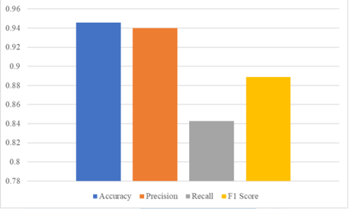
Figure 11 presents the machine learning model's major performance metrics. With a precision of 94.0% and an accuracy of 94.5%, the model shows good overall performance and a low false positive rate. The lower recall number of 84.2% indicates that the model is missing roughly 15.8% of the positive cases it ought to detect, which could be a serious issue depending on the application scenario. The F1-score is 88.9%, which gives the harmonic mean of recall and precision. By balancing the trade-off between recall and precision, this statistic provides a more thorough understanding of model performance than either metric. These findings show that the model performs exceptionally well at correctly identifying the instances it predicts as positive (high accuracy). However, locating all pertinent positive occurrences in the dataset (lower recall) is considerably complex. According to this performance profile, the model might be better suited for applications where erroneous positives are more expensive than false negatives. The disparity between precision and recall in essential security applications, such as those mentioned in the earlier analysis of attack predictions, warrants more research and significantly increases the detection rate of actual attack instances.

Download: Download full-size image

Figure 11. Performance Metrics of the Model.

5. Conclusion

The design and implementation of a platform for advancing cross-domain intrusion detection has been presented. The platform is based on the integration of one-dimensional convolutional neural networks and GloVe embeddings. The design emphasised the synergistic advantages of combining CNN-based feature extraction with the contextual understanding provided by word embeddings. As cyber threats continue to evolve, the proposed platform presents a promising avenue for enhancing the resilience and adaptability of cybersecurity measures in an increasingly complex digital landscape. The implementation of the platform was mainly supported by Visual Studio Code IDE, Python as the programming language, and Streamlit. A one-dimensional convolutional neural network was integrated with GloVe embeddings for advancing cross-domain intrusion detection. The platform emphasises the synergistic advantages of combining CNN-based feature extraction with the contextual understanding provided by word embeddings. The experimental study of the new platform achieved a reliable cross-domain network intrusion detection. The study also showed a very promising avenue for enhancing the resilience and adaptability of cybersecurity measures in an increasingly complex digital landscape. It was also revealed that the 1D-CNN and GloVe embeddings model for cross-domain network intrusion detection led to improved performances of some of the existing network intrusion detection systems.

One limitation of 1D-CNNs is their constrained ability to capture long-range dependencies in text, as the convolutional filters are primarily designed to identify local patterns. This approach restricts the effectiveness of models when contextual relationships extend beyond the immediate vicinity of any given token. In addition, pretrained GloVe embeddings, which are static, fail to account for polysemy and context variations in language use, leading to potential semantic inaccuracies. As language continually evolves, the static embeddings may not represent new usages or domain-specific terminologies effectively. Moreover, 1D-CNN models usually require extensive tuning of hyperparameters such as kernel sizes and filter numbers to achieve optimal performance, potentially resulting in increased computational cost when processing large-scale datasets. These limitations necessitate further research into dynamic embedding models and architectures that integrate long-term contextual understanding.

Abbreviations

DDoS)	Distributed Denial of Service
CSV	Comma-Separated Value
1D-CNN	One-Dimensional Convolutional Neural Network
NIDS	Network Intrusion Detection System
PCA	Principal Component Analysis
APTs	Advanced Persistent Threats
CDIDS	Cross-Domain Intrusion Detection System
IDS	Intrusion Detection Systems
NAEF	Nonlinear Augmented Explicit Features
OSVM	One-Class Support Vector Machine
MLP	Multi-Layer Perceptron
VS	Visual Studio

Author Contributions

Gabriel Babatunde Iwasokun: Conceptualization, Data curation, Formal Analysis, Funding acquisition, Investigation, Supervision, Writing – original draft, Writing – review & editing

Ahmed Ojodu: Conceptualization, Data curation, Formal Analysis

Johnson Adeleke Adeyiga: Methodology, Resources, Validation, Visualization

Oludare Johnson Olaleye: Methodology, Resources, Validation, Visualization

Mojisola Olajumoke Ogunseye: Methodology, Resources, Validation, Visualization

Ibraheem Temitope Jimoh: Methodology, Resources, Validation, Visualization

David Bamidele Adewole: Methodology, Resources, Validation, Visualization

Conflicts of Interest

The authors declares no conflicts of interest.

References

[1]	Almehdhar, M., Albaseer, A., Khan, M. A., Abdallah, M., Menouar, H., Al-Kuwari, S., & Al-Fuqaha, A. (2024). Deep learning in the fast lane: A survey on advanced intrusion detection systems for intelligent vehicle networks. IEEE Open Journal of Vehicular Technology. Available: https://ieeexplore.ieee.org/stamp/stamp.jsp?arnumber=10582439
[2]	Lampe, B., & Meng, W. (2023). Intrusion detection in the automotive domain: A comprehensive review. IEEE Communications Surveys & Tutorials. Available: https://orbit.dtu.dk/files/341095318/Intrusion_Detection_in_the_Automotive_Domain_A_Comprehensive_Review.pdf
[3]	Chen, Y., Su, S., Yu, D., He, H., Wang, X., Ma, Y., & Guo, H. (2022). Cross-domain industrial intrusion detection deep model trained with imbalanced data. IEEE Internet of Things Journal, 10(1), 584-596. https://doi.org/10.1109/JIOT.2022.3201888
[4]	Ali, S., Li, Q., & Yousafzai, A. (2024). Blockchain and federated learning-based intrusion detection approaches for edge-enabled industrial IoT networks: A survey. Ad Hoc Networks, 152, 103320. Available: https://dl.acm.org/doi/10.1016/j.adhoc.2023.103320
[5]	Park, C., Lee, J., Kim, Y., Park, J. G., Kim, H., & Hong, D. (2022). An enhanced AI-based network intrusion detection system using generative adversarial networks. IEEE Internet of Things Journal, 10(3), 2330-2345. https://doi.org/10.1109/JIOT.2022.3211346
[6]	Abu Al-Haija, Q., & Al Badawi, A. (2022). High-performance intrusion detection system for networked UAVs via deep learning. Neural Computing and Applications, 34(13), 10885-10900. Available: https://doi/10.1007.s00521-022-07015-9
[7]	Chang, V., Golightly, L., Modesti, P., Xu, Q. A., Doan, L. M. T., Hall, K., & Kobusińska, A. (2022). A survey on intrusion detection systems for fog and cloud computing. Future Internet, 14(3), 89. Available: https://norma.ncirl.ie/8161/1/mayuriganeshumrikar.pdf
[8]	Laghrissi, F., Hssina, B., Douzi, K., & Douzi, S. (2021). Intrusion detection systems using long short-term memory (LSTM). Journal of Big Data, 8(1). Available: https://thesai.org/Downloads/Volume13No12/Paper_14-Intrusion_Detection_System_using_Long_Short_Term_Memory.pdf
[9]	Dina, A. S., & Manivannan, D. (2021). Intrusion detection based on Machine Learning techniques in computer networks. Internet of Things, 16, 100462. https://doi.org/10.1016/j.iot.2021.100462
[10]	Yu, X., Lu, Y., Jiang, F., Hu, Q., Du, J., & Gong, D. (2024). A Cross-Domain Intrusion Detection Method Based on Nonlinear Augmented Explicit Features. IEEE Transactions on Network and Service Management. https://doi.org/10.1109/TNSM.2024.3444909
[11]	Choi, H., Lee, J., Lee, W., Kwon, Y., Myoung, N., Park, M., & Song, J. J. (2024). Cross-Domain Solution with Stateful Correlation of Outgoing and Incoming Application-Layer Packets. IEEE Access, 12, 26830-26838. Available: https://ieeexplore.ieee.org/stamp/stamp.jsp?arnumber=10439189
[12]	Layeghy, S., & Portmann, M. (2023). Explainable cross-domain evaluation of ML-based network intrusion detection systems. Computers and Electrical Engineering, 108, 108692. https://doi.org/10.1016/j.compeleceng.2023.108692
[13]	Layeghy, S., Baktashmotlagh, M., & Portmann, M. (2023). DI-NIDS: Domain invariant network intrusion detection system. Knowledge-Based Systems, 273, 110626. https://doi.org/10.1016/j.knosys.2023.110626
[14]	Zhang, C., Wang, G., Wang, S., Zhan, D., & Yin, M. (2023). Cross-domain network attack detection enabled by heterogeneous transfer learning. Computer Networks, 227, 109692. https://doi.org/10.1016/j.comnet.2023.109692
[15]	Abdallah, M., Jahromi, H., Delia Jurcut, A., & An Le Khac, N. (2021, August 17). A Hybrid CNN-LSTM-Based Approach for Anomaly Detection Systems in SDNs. https://doi.org/10.1145/3465481.3469190
[16]	Zhang, Z., Theesfeld, C. L., Troyanskaya, O. G., & Park, C. Y. (2021). An automated framework for efficiently designing deep convolutional neural networks in genomics. Nature Machine Intelligence, 3(5), 392-400. Available: https://www.nature.com/articles/s42256-021-00316-z
[17]	Jolliffe, I. T. (2002). Principal Component Analysis (Second Edition). Springer. Available: http://cda.psych.uiuc.edu/statistical_learning_course/Jolliffe%20I.%20Principal%20Component%20Analysis%20(2ed.,%20Springer,%202002)(518s)_MVsa_.pdf
[18]	Bishop, C. M. (2006). Pattern recognition and machine learning. Springer. Available: chrome-extension: //efaidnbmnnnibpcajpcglclefindmkaj/ https://www.microsoft.com/en-us/research/wp-content/uploads/2006/01/Bishop-Pattern-Recognition-and-Machine-Learning-2006.pdf
[19]	Vellela S. S., Roja D., NagaMalleswara R. P., Syamsundara R. T., Lakshma R. V., Ramesh V. (2026). Cyber Threat Detection in Industry 4.0: Leveraging GloVe and Self-Attention Mechanisms in BiLSTM for Enhanced Intrusion Detection, Computers and Electrical Engineering, 124. https://doi.org/10.1016/j.compeleceng.2025.110368
[20]	Kondaiah C., Pais A., & Routhu S. (2025). TrackPhish: A Multi-Embedding Attention-Enhanced 1D CNN Model for Phishing URL Detection. IEEE Transactions on Information Forensics and Security. https://doi.org/10.1109/TIFS.2025.3629558
[21]	Oladejo O, & Ahmed A. A. (2026). Leveraging Cross-Domain Transfer Learning for Enhanced Multi-Protocol Network Intrusion Detection, Computers 2026, 15(6), 376. https://doi.org/10.3390/computers15060376
[22]	Sinha R. (2026). Cross-Domain Evaluation of CNN-Based and Generative Adversarial Networks Models’ Generalisability for (D)DoS Attack Detection in CPS and IoT, https://doi.org/10.1007/978-981-96-7036-9_2

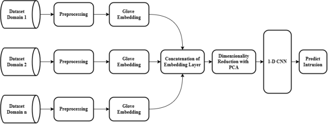
Cite This Article

Plain Text BibTeX RIS

APA Style

Iwasokun, G. B., Ojodu, A., Adeyiga, J. A., Olaleye, O. J., Ogunseye, M. O., et al. (2026). Cross-domain Network Intrusion Detection Based on 1-D CNN, PCA, and GloVe Embedding. American Journal of Networks and Communications, 15(2), 33-48. https://doi.org/10.11648/j.ajnc.20261502.11

Copy | Download

ACS Style

Iwasokun, G. B.; Ojodu, A.; Adeyiga, J. A.; Olaleye, O. J.; Ogunseye, M. O., et al. Cross-domain Network Intrusion Detection Based on 1-D CNN, PCA, and GloVe Embedding. Am. J. Netw. Commun. 2026, 15(2), 33-48. doi: 10.11648/j.ajnc.20261502.11

Copy | Download

AMA Style

Iwasokun GB, Ojodu A, Adeyiga JA, Olaleye OJ, Ogunseye MO, et al. Cross-domain Network Intrusion Detection Based on 1-D CNN, PCA, and GloVe Embedding. Am J Netw Commun. 2026;15(2):33-48. doi: 10.11648/j.ajnc.20261502.11

Copy | Download

@article{10.11648/j.ajnc.20261502.11,
  author = {Gabriel Babatunde Iwasokun and Ahmed Ojodu and Johnson Adeleke Adeyiga and Oludare Johnson Olaleye and Mojisola Olajumoke Ogunseye and Ibraheem Temitope Jimoh and David Bamidele Adewole},
  title = {Cross-domain Network Intrusion Detection Based on 1-D CNN, PCA, and GloVe Embedding},
  journal = {American Journal of Networks and Communications},
  volume = {15},
  number = {2},
  pages = {33-48},
  doi = {10.11648/j.ajnc.20261502.11},
  url = {https://doi.org/10.11648/j.ajnc.20261502.11},
  eprint = {https://article.sciencepublishinggroup.com/pdf/10.11648.j.ajnc.20261502.11},
  abstract = {The existing communication networks are currently encompassed with various malicious activities that aim to compromise the confidentiality, integrity, and availability of data and systems. The activities include malware, phishing, ransomware, Distributed Denial of Service (DDoS) attacks, and insider attacks. The rapid evolution of these threats necessitates the development of advanced and adaptable intrusion detection systems (IDS) capable of operating across diverse network environments. This paper presents the design of a cross-domain network intrusion detection system that leverages a convolutional neural network and principal components analysis to enhance network intrusion detection accuracy and generalisation. The design integrates GloVe (Global Vectors for Word Representation) embeddings to transform network traffic data into a meaningful feature space, utilises Principal Component Analysis (PCA) for dimensionality reduction, and employs a one-dimensional Convolutional Neural Network (1D-CNN) for efficient classification of network activities. The design also considered preprocessing of multiple intrusion detection data from various network domains, and each data is subjected to GloVe-based feature extraction to generate dense vector representations, which are subsequently concatenated to form a unified embedding layer. The PCA component is required for mitigating the issues with dimensionality and enhancing computational efficiency. It will also be used to extract some significant features before the 1D-CNN-enabled intrusion classification. The experimental study of the system established its practical function and suitability for a very high, accurate, and reliable detection of intrusions in multi-domain networks.},
 year = {2026}
}

Copy | Download

TY  - JOUR
T1  - Cross-domain Network Intrusion Detection Based on 1-D CNN, PCA, and GloVe Embedding
AU  - Gabriel Babatunde Iwasokun
AU  - Ahmed Ojodu
AU  - Johnson Adeleke Adeyiga
AU  - Oludare Johnson Olaleye
AU  - Mojisola Olajumoke Ogunseye
AU  - Ibraheem Temitope Jimoh
AU  - David Bamidele Adewole
Y1  - 2026/07/28
PY  - 2026
N1  - https://doi.org/10.11648/j.ajnc.20261502.11
DO  - 10.11648/j.ajnc.20261502.11
T2  - American Journal of Networks and Communications
JF  - American Journal of Networks and Communications
JO  - American Journal of Networks and Communications
SP  - 33
EP  - 48
PB  - Science Publishing Group
SN  - 2326-8964
UR  - https://doi.org/10.11648/j.ajnc.20261502.11
AB  - The existing communication networks are currently encompassed with various malicious activities that aim to compromise the confidentiality, integrity, and availability of data and systems. The activities include malware, phishing, ransomware, Distributed Denial of Service (DDoS) attacks, and insider attacks. The rapid evolution of these threats necessitates the development of advanced and adaptable intrusion detection systems (IDS) capable of operating across diverse network environments. This paper presents the design of a cross-domain network intrusion detection system that leverages a convolutional neural network and principal components analysis to enhance network intrusion detection accuracy and generalisation. The design integrates GloVe (Global Vectors for Word Representation) embeddings to transform network traffic data into a meaningful feature space, utilises Principal Component Analysis (PCA) for dimensionality reduction, and employs a one-dimensional Convolutional Neural Network (1D-CNN) for efficient classification of network activities. The design also considered preprocessing of multiple intrusion detection data from various network domains, and each data is subjected to GloVe-based feature extraction to generate dense vector representations, which are subsequently concatenated to form a unified embedding layer. The PCA component is required for mitigating the issues with dimensionality and enhancing computational efficiency. It will also be used to extract some significant features before the 1D-CNN-enabled intrusion classification. The experimental study of the system established its practical function and suitability for a very high, accurate, and reliable detection of intrusions in multi-domain networks.
VL  - 15
IS  - 2
ER  -

Copy | Download

Author Information

Gabriel Babatunde Iwasokun

Department of Computer Science and Information Technology, Bells University of Technology, Ota, Nigeria; Department of Software Engineering, Federal University of Technology, Akure, Nigeria

Contact Email

http://orcid.org/0000-0002-9775-5631
Ahmed Ojodu

Department of Computer Science and Information Technology, Bells University of Technology, Ota, Nigeria

Contact Email
Johnson Adeleke Adeyiga

Department of Computer Science and Information Technology, Bells University of Technology, Ota, Nigeria

Contact Email

http://orcid.org/0000-0002-3763-490X
Oludare Johnson Olaleye

Department of Computer Science and Information Technology, Bells University of Technology, Ota, Nigeria

Contact Email
Mojisola Olajumoke Ogunseye

Department of Computer Science, Federal University of Technology, Akure, Nigeria

Contact Email

http://orcid.org/0009-0001-3777-1971
Ibraheem Temitope Jimoh

Department of Software Engineering, Federal University of Technology, Akure, Nigeria

Contact Email

http://orcid.org/0009-0005-3426-7162
David Bamidele Adewole

Department of Software Engineering, Federal University of Technology, Akure, Nigeria

Contact Email

http://orcid.org/0009-0001-3382-3025

Download PDF

Submit an Article

Plain Text BibTeX RIS

APA Style

Iwasokun, G. B., Ojodu, A., Adeyiga, J. A., Olaleye, O. J., Ogunseye, M. O., et al. (2026). Cross-domain Network Intrusion Detection Based on 1-D CNN, PCA, and GloVe Embedding. American Journal of Networks and Communications, 15(2), 33-48. https://doi.org/10.11648/j.ajnc.20261502.11

Copy | Download

ACS Style

Iwasokun, G. B.; Ojodu, A.; Adeyiga, J. A.; Olaleye, O. J.; Ogunseye, M. O., et al. Cross-domain Network Intrusion Detection Based on 1-D CNN, PCA, and GloVe Embedding. Am. J. Netw. Commun. 2026, 15(2), 33-48. doi: 10.11648/j.ajnc.20261502.11

Copy | Download

AMA Style

Iwasokun GB, Ojodu A, Adeyiga JA, Olaleye OJ, Ogunseye MO, et al. Cross-domain Network Intrusion Detection Based on 1-D CNN, PCA, and GloVe Embedding. Am J Netw Commun. 2026;15(2):33-48. doi: 10.11648/j.ajnc.20261502.11

Copy | Download

@article{10.11648/j.ajnc.20261502.11,
  author = {Gabriel Babatunde Iwasokun and Ahmed Ojodu and Johnson Adeleke Adeyiga and Oludare Johnson Olaleye and Mojisola Olajumoke Ogunseye and Ibraheem Temitope Jimoh and David Bamidele Adewole},
  title = {Cross-domain Network Intrusion Detection Based on 1-D CNN, PCA, and GloVe Embedding},
  journal = {American Journal of Networks and Communications},
  volume = {15},
  number = {2},
  pages = {33-48},
  doi = {10.11648/j.ajnc.20261502.11},
  url = {https://doi.org/10.11648/j.ajnc.20261502.11},
  eprint = {https://article.sciencepublishinggroup.com/pdf/10.11648.j.ajnc.20261502.11},
  abstract = {The existing communication networks are currently encompassed with various malicious activities that aim to compromise the confidentiality, integrity, and availability of data and systems. The activities include malware, phishing, ransomware, Distributed Denial of Service (DDoS) attacks, and insider attacks. The rapid evolution of these threats necessitates the development of advanced and adaptable intrusion detection systems (IDS) capable of operating across diverse network environments. This paper presents the design of a cross-domain network intrusion detection system that leverages a convolutional neural network and principal components analysis to enhance network intrusion detection accuracy and generalisation. The design integrates GloVe (Global Vectors for Word Representation) embeddings to transform network traffic data into a meaningful feature space, utilises Principal Component Analysis (PCA) for dimensionality reduction, and employs a one-dimensional Convolutional Neural Network (1D-CNN) for efficient classification of network activities. The design also considered preprocessing of multiple intrusion detection data from various network domains, and each data is subjected to GloVe-based feature extraction to generate dense vector representations, which are subsequently concatenated to form a unified embedding layer. The PCA component is required for mitigating the issues with dimensionality and enhancing computational efficiency. It will also be used to extract some significant features before the 1D-CNN-enabled intrusion classification. The experimental study of the system established its practical function and suitability for a very high, accurate, and reliable detection of intrusions in multi-domain networks.},
 year = {2026}
}

Copy | Download

TY  - JOUR
T1  - Cross-domain Network Intrusion Detection Based on 1-D CNN, PCA, and GloVe Embedding
AU  - Gabriel Babatunde Iwasokun
AU  - Ahmed Ojodu
AU  - Johnson Adeleke Adeyiga
AU  - Oludare Johnson Olaleye
AU  - Mojisola Olajumoke Ogunseye
AU  - Ibraheem Temitope Jimoh
AU  - David Bamidele Adewole
Y1  - 2026/07/28
PY  - 2026
N1  - https://doi.org/10.11648/j.ajnc.20261502.11
DO  - 10.11648/j.ajnc.20261502.11
T2  - American Journal of Networks and Communications
JF  - American Journal of Networks and Communications
JO  - American Journal of Networks and Communications
SP  - 33
EP  - 48
PB  - Science Publishing Group
SN  - 2326-8964
UR  - https://doi.org/10.11648/j.ajnc.20261502.11
AB  - The existing communication networks are currently encompassed with various malicious activities that aim to compromise the confidentiality, integrity, and availability of data and systems. The activities include malware, phishing, ransomware, Distributed Denial of Service (DDoS) attacks, and insider attacks. The rapid evolution of these threats necessitates the development of advanced and adaptable intrusion detection systems (IDS) capable of operating across diverse network environments. This paper presents the design of a cross-domain network intrusion detection system that leverages a convolutional neural network and principal components analysis to enhance network intrusion detection accuracy and generalisation. The design integrates GloVe (Global Vectors for Word Representation) embeddings to transform network traffic data into a meaningful feature space, utilises Principal Component Analysis (PCA) for dimensionality reduction, and employs a one-dimensional Convolutional Neural Network (1D-CNN) for efficient classification of network activities. The design also considered preprocessing of multiple intrusion detection data from various network domains, and each data is subjected to GloVe-based feature extraction to generate dense vector representations, which are subsequently concatenated to form a unified embedding layer. The PCA component is required for mitigating the issues with dimensionality and enhancing computational efficiency. It will also be used to extract some significant features before the 1D-CNN-enabled intrusion classification. The experimental study of the system established its practical function and suitability for a very high, accurate, and reliable detection of intrusions in multi-domain networks.
VL  - 15
IS  - 2
ER  -

Copy | Download