Research Article | | Peer-Reviewed

The Distribution of Risk Across Healthcare Providers and Reducing Misclassification

Received: 22 March 2024    Accepted: 7 April 2024    Published: 29 April 2024
Views:       Downloads:
Abstract

Four linear multilevel mixed-risk models were compared using model assumption tests and predictions. Models varied by the number of random intercepts from 1 to 4, producing 2-level through 5-level models of the same measure, operative time. Normality of the dependent variable and residuals, variance homoscedasticity, level-1, and level-2 exogeneity were tested using the robust test of the level-1 residuals variance by surgeon, estimates of density, skew, and the Hausman test. Measure (operative time by hospital and surgeon) aberrancy and risk classification were evaluated using traditional methods and used to assess distribution measures. The dependent variable and the level-1 residuals required transformation for linearity and variance stabilization, respectively. Normality criteria were met for both level-1 and level-2 residuals and standardized residuals. The likelihood ratio comparing the four models was significantly larger for the 5-level (1016.1; P<0.00005) model than the likelihood ratio for the four-level and other models. Shrinkage was greatest for the 2-level model (0.039; P<0.00005) and least for the 5-level model (0.028; P<0.00005). Level-1 variance homoscedasticity was confirmed by the robust variance test across all models (P>F=1). Aberrant value detection did not require the exclusion of any observations, while prediction intervals revealed low or high risk for 54.2% of surgeons for the 2-level model and 8.6% for the 5-level model. The traditional (c2 = -11.01; P=1) and instrumental variable (c2 = 21.06; P=1) Hausman tests show that the null hypothesis cannot be rejected for level-1 or level-2 exogeneity. Once level-1 and level-2 exogeneity was confirmed, and since deconfounding was a model consideration, causal inferential capacity was assumed. The likelihood ratio, residual variance, shrinkage, and predictions show that the 5-level model is preferred to the other models.

Published in American Journal of Theoretical and Applied Statistics (Volume 13, Issue 2)
DOI 10.11648/j.ajtas.20241302.11
Page(s) 29-38
Creative Commons

This is an Open Access article, distributed under the terms of the Creative Commons Attribution 4.0 International License (http://creativecommons.org/licenses/by/4.0/), which permits unrestricted use, distribution and reproduction in any medium or format, provided the original work is properly cited.

Copyright

Copyright © The Author(s), 2024. Published by Science Publishing Group

Keywords

Misclassification, Assumption/Specification Tests, Multi-level Mixed Effects Model, Random Intercept, Confounding, Causal

1. Introduction
One of the main objectives of multilevel mixed modeling is to compute empirical Bayesian means, which represent the means of the posterior distribution or clusters of interest. These clusters can include a range of factors, such as the longitudinal weight of pigs , a comparison of measuring devices , or an evaluation of the performance of hospitals or surgeons . Before 2001, the standard approach to risk modeling included single-level modeling based on the estimated measure; if the measure were a binary outcome, such as mortality, standard logistic regression could be employed . Thus, sample size differences, clustering effects, and reliability were not considered; only patient-level effects were assessed despite their aggregation with effects from other levels such as hospital and surgeon. These method flaws came to be seen as a reporting failure , and recommendations included the use of “multilevel models” and “report formats that emphasize the statistical uncertainty of the results.” Shahian concludes by recommending that other quality markers, including measures of process and structure, be included. The outcome of flawed risk assessments is misclassification due to the acceptance of unreliable or aberrant clusters or model misspecification. In public reporting, misclassification results in mislabeling the risk of a specific hospital or physician as incorrectly low or high for an outcome, such as mortality, or a complication, such as surgical site infection, or a process measure, such as length of stay. In quality improvement, misclassification points in the wrong direction for improvement, resulting in resource misallocation. In the recommended model form, in addition to the traditional dependent variable such as mortality, readmission, or operative time, random intercepts are incorporated to represent additional study variables, such as hospitals or Physicians; however, other institutional or Physician attributes could also be effective as a random intercept, such as inpatient or outpatient status, among others.
This study compares multi-level models to assess surgical outcomes across patients, surgical procedures, surgeons, and hospitals. It aims to improve model performance over the traditional two-level model and reduce risk misclassification. Operative time is an independent measure of risk for postoperative complications . Operative time is also used to assess surgical learning .
2. Methods
The data set used in this study has been previously described. I compared four multilevel mixed linear random intercept models with 2, 3, 4, or 5 levels to risk-adjust operative time for 28,045 surgical cases across 631 surgeons and twenty-three hospitals. Since operative time has a lognormal distribution, it was transformed to eliminate skewness [STATA command "lnskew0"]. All statistical analyses were performed using STATA 17 software . The primary examples in this study are estimates of the risk of long-duration surgical procedures for hospitals and surgeons. This process aims to provide information that the surgeon or hospital could use for quality improvement.

2.1. Model Fitting

Standard demographic, preoperative risk and case-mix variables were included as fixed and random effects in the models using the STATA command "mixed." Random intercepts were added conditionally for inpatient/outpatient status, the number of procedures performed for each patient, and the identification of each hospital and surgeon. The likelihood ratio test (STATA command "lrtest") was used to compare models and determine if adding random intercepts improved model fit. Random intercepts were included only if the diagnostic standard error (dxse) could be calculated for most surgeons. The likelihood ratio test assesses the hypothesis that the random intercept is zero; if true, the random intercept is not helpful. The dxse was chosen because it depends on the difference of the between surgeon variance and the within-surgeon variance (standard error of the surgeon random intercept). However, surgeons with standard errors of the random intercept larger than the between-surgeon variance were excluded because of the need to take the square root of a negative.

2.2. Testing Model Assumptions

Assessment of normality of transformed operative time is by comparison of the kernel density estimate with a normal reference distribution and the normal quantile plot [STATA commands “kdensity” and “qnorm”]. Comparison of the absolute maximum likelihood (ML) random intercepts to the absolute empirical Bayesian predicted random intercepts confirms that the ML version is larger. Absolute values are used because both ML and EB versions can be negative; using absolute values identifies which is furthest from zero for both sides of zero. Level-1 residuals are assumed homoscedastic and evaluated using the median-centered version of Levene’s test to avoid any possible confounding due to skew in their distribution [STATA command “robvar2”]. Level-2 residuals (the random intercepts) are also assumed homoscedastic; however, testing for homoscedasticity is unnecessary, as the random intercept does not vary within group. Normality assumptions for level-1 residuals when n is large, as in this study, are more difficult to confirm due to limitations of normality testing such as the Shapiro-Wilk W test and the Shapiro-Francia W’ test; both for normal data have sample size limitations of 2,000 and 5,000, respectively. Level-1 raw and standardized residuals can be evaluated for normality even though the central limit theorem applies, and normality could be assumed . The formula for standardized residuals results in an asymptotic standard normal distribution. Both raw and standardized residual normality are evaluated by kernel density estimate comparison to a normal reference distribution and estimates of skew [STATA commands, kdensity, and “summarize, detail” or “sktest”]. The best linear unbiased predictions (BLUPS, random intercepts, or level-2 residuals) [STATA command “predict”] are evaluated for aberrancy using the criterion of greater than two diagnostic standard errors. Graphic analysis of aberrancy is facilitated by expressing each random intercept in diagnostic standard errors (dxse) and comparing it against the number of cases in dxse space. While random intercept prediction intervals based on comparative standard errors are used to identify surgeons with either an insignificant or high risk of long-duration procedures, diagnostic standard errors are used to test the assumption that approximately 5 percent of total surgeons should have either high or low operative times. The comparative standard error (cse) is estimated by multiplying (1 - shrinkage factor) by the between surgeon variance (random effect). The dxse is estimated by multiplying the shrinkage factor by the between surgeon variance. Dxse is equal to cse when the shrinkage factor is 0.5, larger than cse when the shrinkage factor is > 0.5, and less than cse when the shrinkage factor is < 0.5. The shrinkage factor is also the reliability of the maximum likelihood random intercept; low reliability, < 50%, identifies clusters where the variance of the prediction errors is greater than the posterior variance. The shrinkage factor can be calculated by dividing the random intercept variance by the sum of the random intercept variance and the level-1 residual variance, where the level-1 variance is divided by the number of cases. The traditional Hausman test is used to compare two different estimators (in this case, fixed effects and or random effects models) of regression coefficients and confirm level-2 homogeneity [STATA command “Hausman”]. The formula for Hausman multiplies both the transposed and the untransposed difference of the two coefficient vectors times the difference of the two covariance matrices; misspecification is confirmed if the two estimators are different. Level-1 errors and time-varying and time-constant covariates are further assessed for exogeneity by comparing the fixed effects and random effects in instrumental variable models [STATA command “xtivreg” followed by “Hausman”] with the Hausman test.
Caterpillar charts identify surgeons and hospitals at low and high risk of long-duration procedures. If more than five percent are classified as having low or high risk, misclassification is assumed. However, the low-risk classification is an innocuous label, and a single-tailed approach could be considered if one has no interest in exemplar identification.
3. Results
The attributes assigned to random intercepts include inpatient/outpatient status, number of surgical procedures performed for each case, hospital ID, and surgeon ID. There are 644 surgeon clusters, fifty-one with just one case and thirty-three with two cases. Random intercepts could not be estimated for thirteen clusters, seven with just one case, two with two cases, and one each with four, nine, ten, and thirteen cases. The maximum likelihood random intercept reliability is less than 0.5 in all clusters with just one case. 2,909 combinations of the four random intercepts used in the 5-level model exist. After also considering aberrancy, there are 587 remaining clusters for analysis. The dependent variable operative time requires transformation to achieve normality as shown in figure 1.
Figure 1. Normality testing of the observed and transformed operative time: Left panel kernel density estimates: untransformed (long dash-dot), transformed (solid line), and reference normal distribution (dash). Right panel normal quantile plot: reference normal (dash) and transformed (circles) showing that the reference normal quantile plot and the transformed value of operative time are nearly identical.

3.1. Likelihood Ratio Comparison

The likelihood ratio comparison of linear multilevel models to ordinary least squares (OLS) regression and the other multilevel models shows that all the multilevel models are better than ordinary least squares, and the 5-level model is preferred to the other multilevel models. Additional random intercepts in this model reduce the residual variance from the 2-level model at 0.14537 (0.14296-0.14783) to 0.14535 (0.14294-0.14780) in the 3-level model, a further reduction to 0.14018 (0.13779-0.14261) in the 4-level model and to 0.13581 (0.13346-0.13820) in the 5-level model. The residual variance can be referred to as the unexplained variance and, as such, reflects goodness of fit. Larger residual variances represent less informative data and greater shrinkage. Based on having the largest likelihood ratio, the 5-level model is preferred to the other models.
Table 1. Comparison of models using the likelihood ratio.

Model

Compared to OLS

Compared to the nested multilevel model

2-level

7305.8*

3-level

7437.7*

2-level = 132*

4-level

10060.4*

3-level = 2622.6*

5-level

11076.5*

4-level = 1016.1*

* P<0.00005

3.2. Comparison of Maximum Likelihood, Empirical Bayesian Random Intercepts, and Shrinkage factors

Reliability-adjustment of the random intercepts occurs in the multilevel mixed modeling process, resulting in the mean differences in the maximum likelihood versus empirical Bayesian values. The adjustment (shrinkage) moves the random intercept value closer to zero. In this case, the 5-level model has the lowest average reliability adjustment (ML-EB), while the 2-level model has the highest average adjustment. These findings comport with residual variance results noted above, where the greatest shrinkage is associated with the largest residual variance.
Table 2. Surgeon-weighted comparison of the absolute maximum likelihood random intercept with the absolute empirical Bayesian random intercept.

Model

Mean difference ML - EB

lower confidence limit

upper confidence limit

t-test ML - EB

Pr (T>t)

Shrinkage factor

2-level

0.039

0.033

0.045

12.7

0.0000

0.863

3-level

0.036

0.03

0.041

13.6

0.0000

0.845

4-level

0.029

0.025

0.034

12.5

0.0000

0.852

5-level

0.028

0.023

0.032

12.2

0.0000

0.856

3.3. Assess for Homoscedasticity of Level-1 Residuals

Table 3. Robust test of equal variances for level-1 residuals by model.

Model

W50

W10

2-level

0.46; P>F=1

0.47; P>F=1

3-level

0.41; P>F=1

0.51; P>F=1

4-level

0.49; P>F=1

0.49; P>F=1

5-level

0.57; P>F=1

0.90; P>F=1

Robust tests for equality of variances for level one residuals show that we cannot reject the null hypothesis that the variances are equal for all models (table 3): residuals were transformed to their reciprocal to stabilize the variance . The W50 is a median-centered version of Levene’s test, and the W10 is the 10% trimmed mean version, which is less sensitive to skew than the standard Levene’s test.

3.4. Normality Testing

Level-1 raw and standardized residuals can be evaluated for normality even though the central limit theorem applies. Both observed (figure 2) and standardized (figure 3) level 1 residual densities have identical shapes. Level 2 residuals (random intercepts) from a linear model are normally distributed as they represent the mean of the posterior distribution (figures 4 and 5).
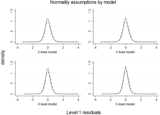
Figure 2. Level 1 residuals are estimated by comparing predicted and observed values. Normality is tested by comparing the densities of the observed and fitted values. These estimated values are represented by the solid line in the density plots above; the dashed line is the reference normal density. The observed densities show a slight skew (0.14 to 0.19).
Figure 3. Standardized level-1 residuals are the level-1 residuals (observed – predicted) multiplied by the inverse square root of the estimated error covariance matrix. Above, the standardized level-1 residuals are represented by the solid line, and the dashed line represents the reference normal distribution. The densities show a slight skew: 0.14 for the 5-level model, 0.15 for the 4-level model, and 0.19 for the two- and 3-level models. The formula for standardized residuals results in an asymptotic standard normal distribution.
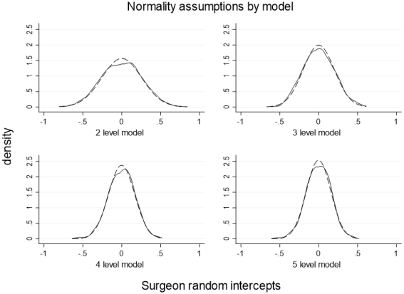
Figure 4. Random intercepts were created in each multilevel model for surgeons. The solid line above represents the observed surgeon random intercepts for each model, while the dashed line is the normal reference distribution. There is a slight skew: 0.05 for the 5-level model, 0.03 for the 4-level model, 0.25 for the 3-level model, and 0.18 for the 2-level model.
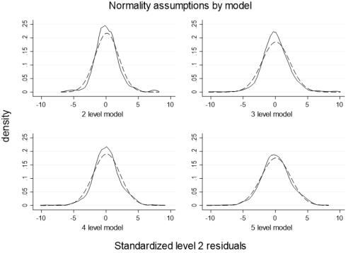
Figure 5. Standardized level 2 residuals are obtained by dividing the random intercepts by the diagnostic standard error; the densities show a slight skew of 0.14 for the 5-level model, 0.16 for the 4-level model, and 0.19 for both the two and 3-level models. The solid lines are the estimated residuals, and the dashed lines are the normal reference distribution.

3.5. Testing for Cluster Aberrancy

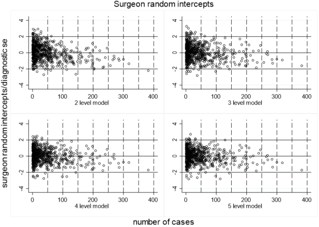
Figure 6. A score created by dividing the random intercepts by the diagnostic standard error aids aberrant value detection by surgeon cluster (each open circle), plotted on the vertical axis against the number of cases per cluster on the horizontal axis. Only 5% of the surgeon clusters should be larger than two dxse. The upper left panel for the 2-level model identifies 29 (4.87%) outlying clusters, and the upper right panel for the 3-level model also identifies twenty-nine outlying clusters. The lower left panel for the 4-level model and the lower right panel for the 5-level model identify 19 (3.2%) outlying clusters. Since there are no models with more than 5% of the random intercepts (surgeon clusters) as outlying, no cases require exclusion from analysis.

3.6. Exogeneity Confirmation

The Hausman tests , and the instrumental variables models confirm level-1 and level-2 exogeneity for both covariate and error types. The traditional Hausman test results showed chi-squared = -11.01, degrees of freedom = 100, and P = 1. This is compelling evidence that we cannot reject the null hypothesis that the random-effects model adequately models the individual-level effects confirming level-2 exogeneity. A positive definite result for the Hausman test is not certain; the negative result reported here can occur in a finite sample because there is nothing to prevent it from being negative when computed in the standard form . The Hausman test for level-1 endogeneity results shows chi-squared = 21.06; degrees of freedom = 96; P = 1.0, that is, the null hypothesis that there is no correlation between the covariates and the level-1 residuals and that level-1 residual expectation is zero cannot be rejected. The lack of correlation with the error term (residuals) means that the x (covariates) vector is exogenous, and the variation in y is the causal treatment effect of x. Similarly, level-2 exogeneity, the lack of correlation between random intercepts and covariate(s), means that the random intercepts do not represent the covariates but an unobserved institutional effect such as the value a hospital inpatient or outpatient setting, or surgeon adds to the patient experience.

3.7. Classification of Risk

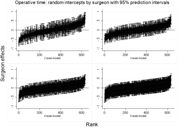
Figure 7. After excluding low reliability and aberrant values and based on random intercepts, the 2-level model caterpillar chart (upper left) identifies 172 surgeons that have a reduced risk of long-duration surgical procedures (LDP) and 151 with an elevated risk; 55% of 587 surgeons are identified as having either high or low risk. The 3-level model chart (upper right) identifies 120 surgeons with a reduced risk of long-duration procedures and 106 with an elevated risk of LDP (38.5%). The lower left chart, the 4-level model, identifies fifty-nine surgeons with a reduced risk of LDP and fifty with a high risk (18.6%). The 5-level model identifies thirty surgeons with a reduced risk of LDP and twenty-one with a high risk (8.7%). There are minor but significant differences in the rank-ordered slopes of the random intercepts shown in the figure above by model: 5-level 0.00085 (0.00082 – 0.00086); 4-level 0.0009005 (0.00087598 – 0.00093); 3-level 0.0011 (0.00106 – 0.0011); 2-level 0.00138 (0.00136 – 0.0014). Additionally, the median standard error of the random intercepts by model is different at 0.08 for the 2-level, 0.088 for the 3-level, 0.12 for the 4-level, and 0.145 for the 5-level model.
The assessment of whether a surgeon or hospital has a high or low risk of long-duration surgical procedures varies widely with the number of random intercepts used to represent institutional attributes of the data. When two random intercepts were used, 54.2% of surgeons were identified as having either low or high risk of long-duration procedures; when four random intercepts were used, only 8.6% of surgeons were identified as having either low or high risk. The four random intercepts used in the five-level model include inpatient status, the number of procedures performed on each patient, a surgeon identifier, and a hospital identifier. A fifth random intercept was assessed in a 6-level model; however, the number of unusable clusters increased since the dxse could not be calculated due to the need to take the square root of a negative. In the modeling process, the four potential random intercepts were used as coefficients when not used as random intercepts in the lower-level models. The effect of missing random intercepts on surgeon-level long-duration surgical procedure risk identification is large. When evaluating hospital performance, it may also be necessary to include surgeon, inpatient or outpatient status, and procedure count random intercepts to reduce misclassification.
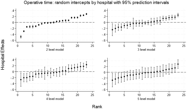
Figure 8. Classification of hospitals for operative time by model: 2 level model shows that 20 of 23 hospitals (87%) are classified as having high (11) or low risk (9) of a long-duration procedure; 3 level model 11 of 23 hospitals (47.8%) are classified as high (5) or low risk (6); 4 level model shows 10 of 23 hospitals (43.5%) are classified as high (5) or low risk (5) and the 5 level model shows 4 hospitals (17.4%) are classified as high (1) or low risk (3). Additionally, the median standard error of the random intercepts by model is different at 0.011 for the 2-level, 0.051 for the 3-level, 0.064 for the 4-level, and 0.085 for the 5-level model.

3.8. Causal Interpretation and Deconfounding

Once strict exogeneity is confirmed, as in this operative time model, coefficients can be interpreted as a causal effect. A variable that is not confounded, body mass index, shows that a one-unit increase in BMI causes a 0.0058 (P < 0.0005) hour (0.35 minutes) increase in operative time. Causal interpretation of regression coefficients is affected by the reasons for their differences: for example, the odds of pneumonia are affected by both operative time and transfusions; the unadjusted (for transfusion) Mantel-Haenszel (M-H) odds (95% confidence interval) of pneumonia are 1.66 (1.55 – 1.77) reflecting conflation of the two causes [STATA command “mhodds”]. However, when adjusted for transfusion, the M-H odds of pneumonia from operative time drop to 1.32 (1.24 – 1.40); the non-overlapping confidence intervals indicate a significant difference. The unadjusted odds include the causal effect of transfusion on pneumonia and the causal effect of operative time on pneumonia and transfusion, in addition to any other unobserved variables. Regression includes all effects in the unadjusted coefficient and can be deconfounded through adjustment for different potential causal factors, such as transfusion. The transfusion rate increases as operative time increases in a general population of surgeries (simple summary linear regression operative time coefficient = 0.033 (0.031-0.035) where transfusion is the dependent variable). The M-H odds of pneumonia due to transfusion and adjusted for operative time is 5.68 (4.59 – 7.0). A separate 5-level logit model of pneumonia shows that the odds of pneumonia due to operative time and transfusion are 1.49 (1.20 – 1.86) and 2.45 (1.88 – 3.19), respectively. The odds ratios reported from the 5-level logit model of pneumonia are preferred as they are adjusted for the entire set of independent variables, not just transfusion or operative time. In the 5-level linear model of operative time, the coefficient for pneumonia when unadjusted for transfusion is 0.048 (0.013 - 0.0835; P = .007); however, adjusting for transfusion lowers the coefficient to 0.029 (-0.005 - 0.065; P = 0.096). Longer duration operative time causes a greater risk of transfusions and pneumonia, while transfusions also cause a greater risk of pneumonia; the directed acyclic graph has an arrow that points from operative time to both transfusion and pneumonia, while transfusion points to pneumonia .
4. Conclusion
Additional random intercepts can improve model performance, as reflected in the likelihood ratio test, residual variance, and risk misclassification. Traditional models focusing on hospitals alone or hospitals and surgeons may experience risk misclassification due to inadequate random effect delivery system classification. However, the estimate of the distribution of risk across surgeons and hospitals and risk misclassification may be adversely impacted by too many random intercepts, as the within-surgeon/hospital variance exceeds the between-surgeon/hospital variance and reliability decreases.
Assumption testing provides a basis for comparing model performance. Causal interpretation in a linear multilevel model requires meeting model assumptions of normality, homoscedastic errors, exogeneity conditions, and deconfounding/deconflation. Confounding implies a level of conflation and unobserved or missing data. In the example of pneumonia, transfusion, and operative time, adjusting for transfusion significantly reduces the size of the coefficient for pneumonia, eliminating conflation and the effect of otherwise missing data.
This study shows that model performance over that of a two-level model using additional random intercepts can be achieved. Random intercepts representing individual characteristics of the patient setting or procedures used, in addition to those traditionally considered, could contribute value to the model, as shown in this example. This approach substantially reduces the risk of misclassification for both hospitals and surgeons.
Author Contributions
William Thomas Cecil is the sole author. The author read and approved the final manuscript.
Conflicts of Interest
The authors declare no conflicts of interest.
References
[1] Ruppert, D., M. P. Wand, and R. J. Carroll. 2003. Semiparametric Regression. Cambridge: Cambridge University Press.
[2] Rabe-Hesketh, S., and A. Skrondal. 2022. Multilevel and Longitudinal Modeling Using Stata. 4th ed. College Station, TX: Stata Press. Based on: J. Martin Bland, Douglas G. Altman. Statistical Methods for Assessing Agreement Between Two Methods of Clinical Measurement. Lancet, 1986; i: 307-310.
[3] Cecil W. T., Selection of Reliable and Valid Surgeon Performance Measures, American Journal of Management Science and Engineering. Volume 5, Issue 5, September 2020, pp. 62-69.
[4] Hannan, Ph. D., E. L., Kilburn, Jr, MA, H., O'Donnell, MA, MS, J. F., Lukacik, MA, G., & Shields, E. (1990). Adult Open Heart Surgery in New York State: An Analysis of Risk Factors and Hospital Mortality Rates. JAMA, 2768 - 2774.
[5] David M. Shahian, Sharon-Lise Normand, David F. Torchiana, Stanley M. Lewis, John O. Pastore, Richard E. Kuntz, Paul I. Dreyer, Cardiac surgery report cards: comprehensive review and statistical critique. This review is an abridged version of a report submitted by the Massachusetts Cardiac Care Quality Commission to the Massachusetts Legislature, May 2001., The Annals of Thoracic Surgery, Volume 72, Issue 6, 2001, Pages 2155-2168, ISSN 0003-4975,
[6] Daley BJ, Cecil W, Clarke PC, Cofer JB, Guillamondegui OD. How slow is too slow? Correlation of operative time to complications: an analysis from the Tennessee Surgical Quality Collaborative. J Am Coll Surg. 2015 Apr; 220(4): 550-8.
[7] Maruthappu, M., Duclos, A., Lipsitz, S. R., Orgill, D., & Carty, M. J. (2015). Surgical learning curves and operative efficiency: A cross-specialty observational study. BMJ Open, 5(3).
[8] StataCorp. 2021. Stata Statistical Software: Release 17. College Station, TX: StataCorp LLC.
[9] Brown, M. B., and A. B. Forsythe. 1974. Robust tests for the equality of variances. Journal of the American Statistical Association 69: 364–367.
[10] Altman, Douglas G. and Bland, Martin J. The normal distribution. British Medical Journal, 310: 298. February 4, 1995.
[11] Wooldridge, Jeffrey M., (2012). Introductory econometrics: a modern approach. Mason, Ohio: South-Western Cengage Learning.
[12] Bland, M. (2015). An Introduction to Medical Statistics (4th ed.). Oxford: Oxford University Press.
[13] Hausman, J. A. 1978. Specification tests in econometrics. Econometrica 46: 1251–1271.
[14] Greene, W. (2018) Econometric Analysis. 8th Edition, Pearson Education Limited, London.
[15] Clayton, D. G., and M. Hills. 1993. Statistical Models in Epidemiology. Oxford: Oxford University Press.
[16] Pearl J. Causality: Models, Reasoning, and Inference. Cambridge University Press, second edition, (2009).
Cite This Article
  • APA Style

    Cecil, W. T. (2024). The Distribution of Risk Across Healthcare Providers and Reducing Misclassification. American Journal of Theoretical and Applied Statistics, 13(2), 29-38. https://doi.org/10.11648/j.ajtas.20241302.11

    Copy | Download

    ACS Style

    Cecil, W. T. The Distribution of Risk Across Healthcare Providers and Reducing Misclassification. Am. J. Theor. Appl. Stat. 2024, 13(2), 29-38. doi: 10.11648/j.ajtas.20241302.11

    Copy | Download

    AMA Style

    Cecil WT. The Distribution of Risk Across Healthcare Providers and Reducing Misclassification. Am J Theor Appl Stat. 2024;13(2):29-38. doi: 10.11648/j.ajtas.20241302.11

    Copy | Download

  • @article{10.11648/j.ajtas.20241302.11,
      author = {William Thomas Cecil},
      title = {The Distribution of Risk Across Healthcare Providers and Reducing Misclassification
    },
      journal = {American Journal of Theoretical and Applied Statistics},
      volume = {13},
      number = {2},
      pages = {29-38},
      doi = {10.11648/j.ajtas.20241302.11},
      url = {https://doi.org/10.11648/j.ajtas.20241302.11},
      eprint = {https://article.sciencepublishinggroup.com/pdf/10.11648.j.ajtas.20241302.11},
      abstract = {Four linear multilevel mixed-risk models were compared using model assumption tests and predictions. Models varied by the number of random intercepts from 1 to 4, producing 2-level through 5-level models of the same measure, operative time. Normality of the dependent variable and residuals, variance homoscedasticity, level-1, and level-2 exogeneity were tested using the robust test of the level-1 residuals variance by surgeon, estimates of density, skew, and the Hausman test. Measure (operative time by hospital and surgeon) aberrancy and risk classification were evaluated using traditional methods and used to assess distribution measures. The dependent variable and the level-1 residuals required transformation for linearity and variance stabilization, respectively. Normality criteria were met for both level-1 and level-2 residuals and standardized residuals. The likelihood ratio comparing the four models was significantly larger for the 5-level (1016.1; PF=1). Aberrant value detection did not require the exclusion of any observations, while prediction intervals revealed low or high risk for 54.2% of surgeons for the 2-level model and 8.6% for the 5-level model. The traditional (c2 = -11.01; P=1) and instrumental variable (c2 = 21.06; P=1) Hausman tests show that the null hypothesis cannot be rejected for level-1 or level-2 exogeneity. Once level-1 and level-2 exogeneity was confirmed, and since deconfounding was a model consideration, causal inferential capacity was assumed. The likelihood ratio, residual variance, shrinkage, and predictions show that the 5-level model is preferred to the other models.
    },
     year = {2024}
    }
    

    Copy | Download

  • TY  - JOUR
    T1  - The Distribution of Risk Across Healthcare Providers and Reducing Misclassification
    
    AU  - William Thomas Cecil
    Y1  - 2024/04/29
    PY  - 2024
    N1  - https://doi.org/10.11648/j.ajtas.20241302.11
    DO  - 10.11648/j.ajtas.20241302.11
    T2  - American Journal of Theoretical and Applied Statistics
    JF  - American Journal of Theoretical and Applied Statistics
    JO  - American Journal of Theoretical and Applied Statistics
    SP  - 29
    EP  - 38
    PB  - Science Publishing Group
    SN  - 2326-9006
    UR  - https://doi.org/10.11648/j.ajtas.20241302.11
    AB  - Four linear multilevel mixed-risk models were compared using model assumption tests and predictions. Models varied by the number of random intercepts from 1 to 4, producing 2-level through 5-level models of the same measure, operative time. Normality of the dependent variable and residuals, variance homoscedasticity, level-1, and level-2 exogeneity were tested using the robust test of the level-1 residuals variance by surgeon, estimates of density, skew, and the Hausman test. Measure (operative time by hospital and surgeon) aberrancy and risk classification were evaluated using traditional methods and used to assess distribution measures. The dependent variable and the level-1 residuals required transformation for linearity and variance stabilization, respectively. Normality criteria were met for both level-1 and level-2 residuals and standardized residuals. The likelihood ratio comparing the four models was significantly larger for the 5-level (1016.1; PF=1). Aberrant value detection did not require the exclusion of any observations, while prediction intervals revealed low or high risk for 54.2% of surgeons for the 2-level model and 8.6% for the 5-level model. The traditional (c2 = -11.01; P=1) and instrumental variable (c2 = 21.06; P=1) Hausman tests show that the null hypothesis cannot be rejected for level-1 or level-2 exogeneity. Once level-1 and level-2 exogeneity was confirmed, and since deconfounding was a model consideration, causal inferential capacity was assumed. The likelihood ratio, residual variance, shrinkage, and predictions show that the 5-level model is preferred to the other models.
    
    VL  - 13
    IS  - 2
    ER  - 

    Copy | Download

Author Information
  • Independent Consultant, Knoxville, United States

  • Abstract
  • Keywords
  • Document Sections

    1. 1. Introduction
    2. 2. Methods
    3. 3. Results
    4. 4. Conclusion
    Show Full Outline
  • Author Contributions
  • Conflicts of Interest
  • References
  • Cite This Article
  • Author Information