Linking Traffic Microsimulation to a Power-Based Vehicle Model to Assess How Operating Regimes Affect Fuel Use and Brake Wear of Diesel, CNG and Electric City Buses

Ulugbek Mamirov Xabibulayevich

doi:doi:10.11648/j.eas.20261105.15

Research Article |

| Peer-Reviewed

Linking Traffic Microsimulation to a Power-Based Vehicle Model to Assess How Operating Regimes Affect Fuel Use and Brake Wear of Diesel, CNG and Electric City Buses

Ulugbek Mamirov Xabibulayevich^*

Published in Engineering and Applied Sciences (Volume 11, Issue 5)

Received: 9 October 2026 Accepted: 20 October 2026 Published: 31 October 2026

Views: Downloads:

Download PDF

Share This Article

Twitter
Linked In
Facebook

Abstract

Traffic engineers routinely use microsimulation to compare bus priority measures, but they report the results almost exclusively as travel time and delay. What happens to the bus itself — its fuel or energy use, the work done by its brakes, the load on its powertrain — is rarely calculated, although these quantities decide the operator's costs. This study closes part of that gap. Driving cycles of a typical Namangan bus corridor (10.4 km, 25 stops, 12 signalised junctions) were generated from PTV Vissim outputs for five operating regimes: the current schedule-based service, an optimised timetable, a shorter headway, conditional transit signal priority (TSP) and an integrated regime. The cycles were fed into a power-based longitudinal model of three 12-m buses: diesel, compressed natural gas (CNG) and battery-electric. The model accounts for passenger load, auxiliary power and, for the electric bus, regenerative braking. In the current regime the diesel bus used 39.3 L/100 km; 35% of the time was spent standing, and 46% of the positive traction energy was later dissipated in the brakes. A decomposition showed that 44.5% of the fuel was time-related (idling and auxiliaries) and 32.6% was spent during acceleration, which occupied only one-tenth of the time. The integrated regime raised the operating speed from 14.3 to 17.1 km/h and reduced consumption by 13.5% for the diesel bus, 13.4% for the CNG bus and 11.7% for the electric bus; TSP alone gave 8.3–9.6%. Brake energy fell by 18%, which corresponds to an estimated 22% longer pad life. A regression fitted to 260 simulated cycles, Q = 10.20 + 0.0601τ + 0.0601 n_st v_c² + 8.05γ (R² = 0.894), reproduces fuel use from three route descriptors with a mean error of 2.2%, and its coefficients agree with their physical estimates within 2–10%. When off-peak hours are included the daily saving of the integrated regime falls to about 10%. The results show that bus priority measures should be appraised by their effect on the number of stops per kilometre, not only by travel time, and that fuel norms for city buses could be made route-specific with little extra data.

Published in	Engineering and Applied Sciences (Volume 11, Issue 5)
DOI	10.11648/j.eas.20261105.15
Page(s)	205-213
Creative Commons	This is an Open Access article, distributed under the terms of the Creative Commons Attribution 4.0 International License (http://creativecommons.org/licenses/by/4.0/), which permits unrestricted use, distribution and reproduction in any medium or format, provided the original work is properly cited.
Copyright	Copyright © The Author(s), 2026. Published by Science Publishing Group

Keywords

City Bus, Fuel Consumption, Energy Consumption, Driving Cycle, Microsimulation, Transit Signal Priority, Brake Wear, Electric Bus

1. Introduction

Fuel and energy are the largest variable costs of urban bus operation, and they depend strongly on how a bus is driven through traffic. The same 12-m bus can use 30 L/100 km on a suburban route and well over 50 L/100 km in a dense centre; field-calibrated bus fuel models show how strongly consumption follows the speed and acceleration profile of the route

[1, 2]

. In our view, this sensitivity is both a problem and an opportunity. It is a problem because fuel norms based on a single figure per vehicle model misrepresent most routes. It is an opportunity because traffic measures — signal priority, timetable changes, stop consolidation — change the driving cycle and can therefore save energy without any change to the vehicle.

Two research traditions deal with this, and they rarely meet. Traffic engineering uses microscopic simulators such as PTV Vissim

[3]

to compare bus priority schemes, including in mixed traffic similar to that of Central Asian cities

[4]

. The outputs are trip times, delays and queues. Vehicle engineering, on the other hand, has well-tested models of fuel use. Wang and Rakha calibrated a power-based model for conventional diesel buses on field data

[1]

; Yu et al. extended the vehicle specific power approach with the passenger load factor and showed that ignoring load biases bus fuel estimates

[2]

; Yang and Liu found in a vehicle–engine simulation that most of the extra energy due to passenger load is spent in the acceleration phase

[5]

. For electric buses, energy demand has been modelled from real-world operating data

[6]

, with physically detailed models that include the thermal load of the cabin

[7, 8]

, and with regression models fitted to fleet measurements

[9]

. These models need exactly the trajectories that microsimulation produces, yet in practice the two are seldom connected. When they are, the vehicle is usually a generic passenger car, and the bus-specific features that matter most — passenger load, auxiliary power for air conditioning, automatic transmission losses, regenerative braking — are dropped.

The question is practical in Uzbekistan. Namangan, a city of over 700,000 people in the Fergana Valley, renewed its bus fleet in 2024–2026 with diesel, gas-powered and, most recently, electric buses operating under gross-cost contracts

[10, 11]

. Fuel norms, however, are still set by fleet-wide coefficients that do not reflect route conditions, and decisions on signal priority are argued in terms of passenger time only. Summer temperatures above 40 °C add another factor: air conditioning can draw 10–20 kW, a load that is large compared with the power needed to keep a bus moving at city speeds.

This paper connects a calibrated Vissim corridor model with a power-based model of three 12-m buses and asks three questions. How do operating regimes change the composition of the driving cycle? How much fuel or energy, brake work and powertrain load do they save for each propulsion type? And can the result be condensed into a simple formula that operators could use to set route-specific fuel norms? Our hypothesis is that the number of stops per kilometre and the time spent per kilometre explain most of the variation, so that measures which remove stops — rather than merely speed up running — deliver the largest vehicle-side benefits.

2. Materials and Methods

2.1. Corridor and Operating Regimes

The study corridor represents a typical bus route in central Namangan: 10.4 km long, with 25 stops (mean spacing 416 m) and 12 signalised junctions. A macroscopic PTV Visum model of the city (150 internal and 11 external zones, 37 bus routes) supplied the passenger loads; a PTV Vissim model of the corridor reproduced traffic, signals, stops and dwell times. The Vissim model was calibrated against traffic counts at 12 junctions (mean GEH statistic 3.7) and against observed travel times (mean deviation 9.2%)

[12]

. Five operating regimes were simulated in Vissim with ten random seeds each (Table 1). The regimes differ in the probability that a bus stops at a signal, the waiting time at signals, the dwell time at stops and the load factor γ, defined as the ratio of passengers on board to nominal capacity.

Table 1. Operating regimes and the resulting operating speed (Vissim output and vehicle model).

Regime	Stop probability at signals	Mean signal wait, s	Mean dwell, s	Load factor γ	Speed, Vissim, km/h	Speed, model, km/h
S1 Current schedule	0.55	32	28	0.62	14.2	14.3
S2 Optimised timetable	0.52	30	23	0.58	15.1	15.0
S3 Shorter headway	0.52	30	19	0.48	15.8	15.6
S4 Conditional TSP	0.10	15	24	0.60	16.5	16.3
S5 Integrated	0.12	15	19	0.50	17.3	17.1

Operating speed includes dwell time. Model speeds are means of ten generated cycles.

2.2. From Vissim Output to Driving Cycles

Vissim can export second-by-second vehicle records for every bus. These records are the natural input for a vehicle model, but running Vissim for every combination of parameters in a sensitivity study is slow. We therefore used Vissim in two ways. The vehicle records were used to estimate the statistical properties of the bus cycle — the stop probability at each signal, the distribution of signal waits and dwell times, and the frequency of congestion slow-downs. A stochastic cycle generator then reproduced cycles with these properties. Signal stops follow a Bernoulli law, signal waits an exponential law, dwell times a gamma law with shape parameter 4, and slow-downs a Poisson process. Between stops the bus accelerates according to

a (v) = \min \{a_{0} (1 - \frac{v}{v_{c} + 8}), \frac{F_{k, \max} (v) - F_{f} - F_{w}}{δ m}\}

(1)

where a₀ = 1.15 m/s² is the initial acceleration, v_c the cruising speed, F_k,max the maximum tractive force, F_f and F_w the rolling and aerodynamic resistance, δ the rotating-mass factor and m the vehicle mass. The first term mimics the desired-acceleration function of Vissim; the second is the traction limit. Deceleration is 1.0 m/s². The only calibrated parameter, the mean cruising speed, was fixed at 25 km/h so that the generator matched the Vissim speed of S1; it was then kept unchanged. The other regimes differ only in their traffic parameters, and the generator still reproduced their Vissim speeds within 1.3% (Table 1). We regard this as the main check of the method.

2.3. Vehicle Model

Three 12-m buses were modelled (Table 2). Their parameters are based on manufacturer data for the Isuzu Citiport 12

[13]

and the Yutong E12

[14]

; the CNG bus represents the 12-m gas-powered buses used in Uzbek cities. Values not published by manufacturers, such as curb mass and idle fuel power, were estimated and are treated as uncertain in Section 3.5.

Table 2. Main parameters of the modelled buses.

Parameter	Diesel	CNG	Electric
Curb mass, kg	11,600	12,200	13,300
Capacity, passengers	85	85	80
Maximum power, kW	224	228	240
Rolling coefficient f₀	0.0090	0.0090	0.0085
C_xA, m²	4.97	4.97	4.62
Driveline efficiency	0.88	0.88	0.85
Auxiliary power, kW	6	6	7
Idle fuel power, kW	12	15	–
Marginal engine efficiency	0.42	0.34	–

The electric bus has a 375 kWh battery and regenerates up to 150 kW at an efficiency of 0.65.

Mass depends on the load factor, m = m₀ + 68 q γ, where q is the capacity and 68 kg the design mass of a passenger. Power at the wheels follows the tractive balance:

P_{w} = [δma + mgf (v) + 0.5 ρ C_{x} A v^{2}] v, f (v) = f_{0} (1 + \frac{v^{2}}{20000})

(2)

For the diesel and CNG buses, fuel power is described by a Willans line, a linear relation between engine output and fuel input; this is the same power-based structure used in recent bus fuel models

[1]

, here with a penalty at high load:

N_{T} = N_{x} + \frac{P_{e}}{η_{m} [1 - 0.22 {(P_{e} / P_{\max})}^{2}]}, P_{e} = \frac{\max (P_{w}, 0)}{η_{tr}} + P_{aux}

(3)

where N_x is the idle fuel power, η_m the marginal efficiency, η_tr the driveline efficiency and P_aux the auxiliary power. During braking the fuel power is set to 0.8 N_x. For the electric bus the battery power is the traction power divided by the driveline efficiency, minus the regenerated part of braking power above 2 m/s, plus auxiliaries. All braking power not regenerated is assumed to be dissipated in the friction brakes. Since friction-brake wear grows with the energy dissipated in the brakes, a relation also used in studies of brake wear emissions

[15]

, pad life was taken as inversely proportional to the friction energy per kilometre and scaled so that the diesel bus in S1 reaches 40,000 km, a typical figure for front pads of city buses.

2.4. Statistical Treatment

Each regime and bus type was evaluated with ten cycles generated from the same set of random seeds, so that differences between regimes are not blurred by different random draws. A Welch t-test was used for pairwise comparisons. To derive a simple predictive formula, 260 additional cycles were generated with randomly varied traffic parameters (signal stop probability 0.05–0.70, signal wait 10–40 s, dwell 12–35 s, 0.3–1.6 slow-downs per km, γ = 0.1–1.0, cruising speed 20–32 km/h).

3. Results

3.1. How the Driving Cycle Changes

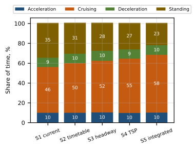
The current regime produces a cycle that is hard on a bus. The diesel bus stops 3.1 times per kilometre and stands still for 35% of the time; it cruises for only 46% of the time (Figure 1). Accelerations and decelerations together take about 19% of the time in all regimes, because they are tied mainly to the number of bus stops, which does not change. What does change is the balance between standing and cruising. The timetable and headway regimes (S2, S3) shorten dwell times but leave the number of stops almost unchanged at 3.07 per km. Signal priority (S4) is the only measure that removes stops: the rate falls to 2.52 per km, a reduction of 18.7%. In the integrated regime (S5) standing time falls to 22.7% and cruising rises to 58%.

Download: Download full-size image

Figure 1. Share of driving time in four operating modes for the diesel bus under the five regimes.

3.2. Fuel and Energy Use

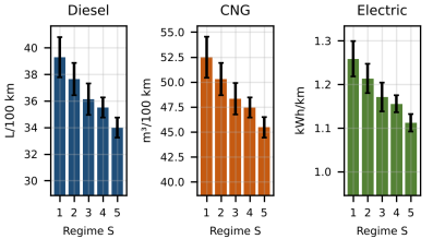
Table 3 and Figure 2 give the results for the three buses. For the diesel bus consumption falls from 39.3 L/100 km in S1 to 34.0 L/100 km in S5, a reduction of 13.5% (t = 9.8, p < 0.001). The CNG bus shows almost the same relative saving, 13.4%. The electric bus saves less, 11.7%, for a reason that is worth spelling out: it consumes nothing but auxiliary power while standing, and it recovers part of the braking energy — 0.206 kWh/km in S1, or about one-sixth of its consumption. A cycle with many stops therefore penalises it less than it penalises a combustion engine.

Table 3. Fuel or energy use and tank-to-wheel or grid CO₂ emissions.

Regime	Diesel, L/100 km	CNG, m³/100 km	Electric, kWh/km	Diesel CO₂, g/km	Electric CO₂*, g/km
S1	39.3 ± 1.5	52.5 ± 2.1	1.26 ± 0.04	1053	629
S2	37.6 ± 1.2	50.3 ± 1.6	1.21 ± 0.03	1009	607
S3	36.1 ± 1.2	48.3 ± 1.6	1.17 ± 0.03	968	586
S4	35.5 ± 0.8	47.4 ± 1.0	1.16 ± 0.02	952	578
S5	34.0 ± 0.8	45.5 ± 1.0	1.11 ± 0.02	911	556

Values are means ± standard deviation of ten cycles. *Assuming a grid factor of 0.50 kg CO₂/kWh, which should be replaced by the current national value.

Download: Download full-size image

Figure 2. Fuel or energy use of the three buses under the five regimes (error bars: ±1 standard deviation).

The difference between S3 and S4 is not statistically significant for the diesel bus (0.6 L/100 km, p ≈ 0.18). The two measures save similar amounts of fuel but in different ways: the shorter headway reduces dwell time and load, while TSP removes accelerations. This distinction matters when the measures are compared per passenger. A shorter headway means more bus-kilometres and lighter buses, so fuel per passenger-kilometre rises: from 0.75 L per 100 passenger-km in S1 to 0.89 in S3. TSP lowers it to 0.70. Viewed from the operator's side, then, a shorter headway is not an energy measure at all unless it is combined with priority.

The propulsion types also differ in absolute terms. In S1 the final energy use is 14.1 MJ/km for the diesel bus, 17.8 MJ/km for the CNG bus and 4.5 MJ/km for the electric bus at the charging point. The CNG bus emits only 2.3% less CO₂ than the diesel bus, because the lower carbon content of natural gas is almost offset by the lower efficiency of the gas engine.

3.3. Where the Fuel Goes

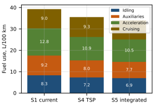
To see which mechanism each measure acts on, the diesel bus's consumption was split into four components (Figure 3). In S1, idling accounts for 21.1% and auxiliaries for 23.4%: 44.5% of the fuel depends on time rather than distance. Acceleration consumes 32.6% while occupying only about 10% of the time. Cruising takes the remaining 22.9%. Between S1 and S5 the time-related part falls by 16.7% and the acceleration part by 18.0%, whereas the cruising part hardly changes (−0.9%). The message is simple. City-bus fuel is saved by cutting time per kilometre and the number of stops; the speed at which the bus cruises between stops is secondary.

Download: Download full-size image

Figure 3. Decomposition of diesel fuel use into idling, auxiliary, acceleration and cruising components.

3.4. A Formula for Fuel Use

The decomposition suggests a formula with three terms — one proportional to time, one to the kinetic energy lost at stops and one to mass:

Q = b_{0} + b_{1} τ + b_{2} n_{st} v_{c}^{2} + b_{3} γ

(4)

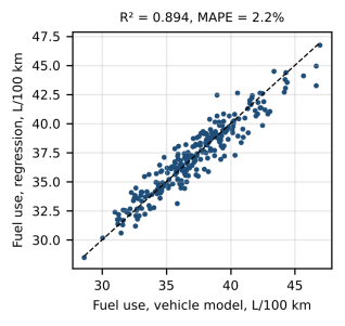
where τ = 3600/V_e is the time per kilometre (s/km), V_e the operating speed, n_st the stops per kilometre and v_c the cruising speed in m/s. Fitted to the 260 cycles, the coefficients are b₀ = 10.20, b₁ = 0.0601, b₂ = 0.0601 and b₃ = 8.05 (Table 4), with R² = 0.894 and a mean absolute percentage error of 2.2% (Figure 4).

Table 4. Regression coefficients for the diesel bus (n = 260).

Coefficient	Estimate	Standard error	t	Physical estimate
b₀, L/100 km	10.20	0.87	11.7	≈ 7.9 (rolling resistance of empty bus)
b₁, (L/100 km)/(s/km)	0.0601	0.0031	19.3	0.073 (idling + auxiliaries)
b₂, (L/100 km)/(m²/s²)	0.0601	0.0018	33.0	0.059 (re-acceleration)
b₃, L/100 km	8.05	0.26	31.4	≈ 7.4 (passenger mass)

R² = 0.894; F = 721; RMSE = 1.06 L/100 km.

Download: Download full-size image

Figure 4. Fuel use from the regression against fuel use from the full vehicle model.

The coefficients are not just fitted numbers. The physical estimate of b₂, the fuel needed to bring the bus back to cruising speed after a stop, is δm/(2η_trη_mH_u) ≈ 0.059 for a mean mass of 14.8 t, within 2% of the fitted value. The fitted b₁ is somewhat lower than its physical estimate, probably because part of the standing time coincides with engine braking in the generated cycles. In practical terms, one avoided signal stop saves about 0.6 mL of diesel per second of waiting and about 29 mL for re-acceleration — roughly 50 mL per stop.

3.5. Brakes, Powertrain Load and Sensitivity

In S1 the diesel bus puts 2.83 MJ/km of positive energy into the wheels and dissipates 1.31 MJ/km in the brakes. Brake energy falls by 14.6% under TSP and by 17.9% under the integrated regime, which corresponds to an estimated pad life of 46,800 and 48,700 km instead of 40,000 km (Table 5). Thanks to regeneration, the electric bus dissipates only 0.28 MJ/km in its friction brakes, about one-fifth of the diesel figure; its estimated pad life approaches 190,000–230,000 km, which suggests that brake service intervals for electric buses could be lengthened.

Table 5. Friction brake energy and estimated pad life.

Regime	Diesel brake energy, MJ/km	Diesel pad life, 10³ km	CNG pad life, 10³ km	Electric pad life, 10³ km
S1	1.31	40.0	38.5	188
S4	1.12	46.8	45.0	224
S5	1.08	48.7	46.8	231

Pad life scaled to 40,000 km for the diesel bus in S1.

Driving style matters as much as the regime for the powertrain. Raising the initial acceleration from 1.15 to 1.5 m/s² increased the operating speed by only 1.4% but raised a fatigue-oriented load index (the mean of the cubed relative engine power) by 66%; lowering it to 0.8 m/s² cut the index by 44% at the cost of 2.1% in speed. Fuel use changed by less than 1% in both directions.

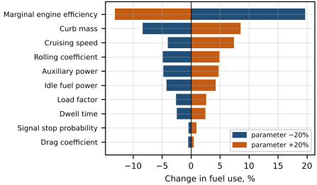
The model is most sensitive to parameters that are hard to measure (Figure 5). A 20% error in the marginal engine efficiency changes fuel use by −13% to +20%; curb mass, cruising speed, rolling resistance, auxiliary power and idle fuel power follow with 4–8%. For comparisons between regimes these errors largely cancel, because they affect all regimes in the same direction. For absolute values they do not, which is why the model must be calibrated against measured fuel use before it is used to set norms.

Download: Download full-size image

Figure 5. Sensitivity of diesel fuel use to a ±20% change in model parameters (regime S1).

4. Discussion

The results support our starting hypothesis. Measures that remove stops deliver the largest vehicle-side savings, and the gain is concentrated in the acceleration and idling components of fuel use. This agrees with the power-based view of bus fuel consumption

[1]

, in which each stop carries a fuel "price" proportional to the kinetic energy that must be restored, and with Yang and Liu's observation that the acceleration phase carries most of the load-related energy penalty

[5]

; in our decomposition the acceleration component also responded most strongly to the regimes. Studies of electric buses report that cycle characteristics and auxiliary loads, rather than speed alone, drive energy demand

[6, 8]

. Our regression in Equation (4) is close in spirit to the multiple linear regression of Sennefelder et al., who reported over 85% prediction accuracy on fleet data from Seville

[9]

; the difference is that our explanatory variables come from a traffic model, so they can be changed by a traffic measure before it is built. What our results add is a direct link from the traffic measures that cities actually debate — signal priority, timetables, headways — to the fuel bill of the operator and to brake wear.

Two findings run against common expectations. The first concerns headways. A shorter headway improves service and, per bus-kilometre, slightly reduces fuel use, because lighter buses dwell for less time. Per passenger-kilometre, however, it increases fuel use by almost 20% in our corridor. This is not an argument against frequent service; it is an argument for combining it with priority so that the extra buses at least run efficiently. The second concerns electric buses. Their relative saving from traffic measures is the smallest of the three types, but in hot weather the measures matter more for them than the percentages suggest. With 16 kW of air conditioning, consumption in S1 rises to about 1.9 kWh/km, and the usable range of a 375-kWh battery falls below 200 km. Detailed thermal models suggest that the cabin load depends on occupancy, door openings and solar gain

[7]

; our constant 16 kW is therefore a coarse assumption, but the direction of the effect is not in doubt. Faster operation in S5 restores part of that margin, which can decide whether a bus completes its daily duty without opportunity charging.

The study has clear limitations. The bus parameters are partly estimated, and the absolute fuel values need confirmation from the operators' records before they can be used as norms. The CO₂ figures for the electric bus depend on the grid factor, which we assumed. Pad life was estimated from friction energy alone and ignores temperature effects, retarders and engine braking; on the flat streets of Namangan this is acceptable, but on hilly routes it is not. The results refer to the morning peak; when off-peak hours, which account for about two-thirds of daily bus-kilometres, are included, the daily saving of the integrated regime for the diesel bus falls from 13.5% to about 10%. Finally, the corridor is a generalised one. For a real route the cruising speed in Equation (4) should be taken from GPS data, because routes with many slow segments would otherwise be overestimated.

Despite these caveats, the approach is cheap to apply. A transport department that already runs Vissim, as Namangan does, can export vehicle records at no extra cost, and the regression in Equation (4) needs only three route descriptors that any GPS dispatch system can provide. Route-specific fuel norms derived in this way would be fairer to drivers and operators than the fleet-wide coefficients in use today.

5. Conclusions

Linking traffic microsimulation with a power-based vehicle model makes the effects of bus priority measures on fuel or energy use, brake work and powertrain load measurable, not just their effects on travel time.

On a typical Namangan corridor, the current regime makes a diesel bus stand still for 35% of the time; 44.5% of its fuel is spent on idling and auxiliaries and 32.6% on accelerations.

Conditional signal priority was the most effective single measure because it was the only one that removed stops. Combined with timetable and headway measures, it reduced peak-hour consumption by 13.5% for a diesel bus, 13.4% for a CNG bus and 11.7% for an electric bus, and cut brake energy by about 18%.

Fuel use of a diesel city bus can be predicted from time per kilometre, stops per kilometre with cruising speed, and load factor with a mean error of about 2%, and the coefficients of the formula have a clear physical meaning. The formula offers a practical basis for route-specific fuel norms.

Future work will calibrate the vehicle model against fuel and energy records of the Namangan fleet and apply the method to real routes using GPS and fare-payment data.

Abbreviations

CNG	Compressed Natural Gas
TSP	Transit Signal Priority
GEH	Geoffrey E. Havers Statistic for Comparing Modelled and Observed Traffic Volumes
RMSE	Root Mean Square Error
CO₂	Carbon Dioxide

Author Contributions

Ulugbek Mamirov is the sole author. The author read and approved the final manuscript.

Conflicts of Interest

The author declares no conflicts of interest.

References

[1]	Wang, J., Rakha, H. A. Fuel Consumption Model for Conventional Diesel Buses. Applied Energy. 2016, 170, 394–402. https://doi.org/10.1016/j.apenergy.2016.02.124
[2]	Yu, Q., Li, T., Li, H. Improving Urban Bus Emission and Fuel Consumption Modeling by Incorporating Passenger Load Factor for Real World Driving. Applied Energy. 2016, 161, 101–111. https://doi.org/10.1016/j.apenergy.2015.09.096
[3]	PTV Group. PTV Vissim 2024 User Manual. Karlsruhe: PTV Planung Transport Verkehr GmbH; 2024.
[4]	Ghosh, T., Bhattacharyya, K., Maitra, B. Traffic Micro-Simulation-Based Evaluation of Bus Priority with Queue Jump Lane on an Urban Corridor with Heterogeneous Traffic Operations. Transportation Research Record. 2022. https://doi.org/10.1177/03611981221090935
[5]	Yang, X., Liu, L. Analysis of the Influence of Passenger Load on Bus Energy Consumption: A Vehicle-Engine Combined Model-Based Simulation Framework. Scientific Reports. 2022, 12, 14535. https://doi.org/10.1038/s41598-022-18866-6
[6]	Gallet, M., Massier, T., Hamacher, T. Estimation of the Energy Demand of Electric Buses Based on Real-World Data for Large-Scale Public Transport Networks. Applied Energy. 2018, 230, 344–356.
[7]	Basma, H., Mansour, C., Haddad, M., Nemer, M., Stabat, P. Comprehensive Energy Modeling Methodology for Battery Electric Buses. Energy. 2020, 207.
[8]	Vepsäläinen, J., Otto, K., Lajunen, A., Tammi, K. Computationally Efficient Model for Energy Demand Prediction of Electric City Bus in Varying Operating Conditions. Energy. 2019, 169, 433–443.
[9]	Sennefelder, R. M., Martín-Clemente, R., González-Carvajal, R. Energy Consumption Prediction of Electric City Buses Using Multiple Linear Regression. Energies. 2023, 16(11), 4365. https://doi.org/10.3390/en16114365
[10]	Gazeta.uz. 12 Buses Delivered for Namangan Public Transport. Available from: https://www.gazeta.uz/oz/2026/07/14/bus-namangan/ (accessed 3 October 2026).
[11]	Yuz.uz. New Electric Buses to Be Put into Service in Namangan. Available from: https://yuz.uz/uz/news/namanganda-yangi- (accessed 3 October 2026).
[12]	Transportation Research Board. Highway Capacity Manual: A Guide for Multimodal Mobility Analysis, 7th ed. Washington, DC: Transportation Research Board; 2022.
[13]	Anadolu Isuzu. Citiport 12: Technical Specifications. Available from: https://www.isuzu.com.tr/en/models/euro5/citiport-12 (accessed 3 October 2026).
[14]	Yutong Bus Co. E12 Electric City Bus. Available from: https://en.yutong.com/products/E12.shtml (accessed 3 October 2026).
[15]	Grigoratos, T., Martini, G. Brake Wear Particle Emissions: A Review. Environmental Science and Pollution Research. 2015, 22(4), 2491–2504. https://doi.org/10.1007/s11356-014-3696-8

Cite This Article

Plain Text BibTeX RIS

APA Style

Xabibulayevich, U. M. (2026). Linking Traffic Microsimulation to a Power-Based Vehicle Model to Assess How Operating Regimes Affect Fuel Use and Brake Wear of Diesel, CNG and Electric City Buses. Engineering and Applied Sciences, 11(5), 205-213. https://doi.org/10.11648/j.eas.20261105.15

Copy | Download

ACS Style

Xabibulayevich, U. M. Linking Traffic Microsimulation to a Power-Based Vehicle Model to Assess How Operating Regimes Affect Fuel Use and Brake Wear of Diesel, CNG and Electric City Buses. Eng. Appl. Sci. 2026, 11(5), 205-213. doi: 10.11648/j.eas.20261105.15

Copy | Download

AMA Style

Xabibulayevich UM. Linking Traffic Microsimulation to a Power-Based Vehicle Model to Assess How Operating Regimes Affect Fuel Use and Brake Wear of Diesel, CNG and Electric City Buses. Eng Appl Sci. 2026;11(5):205-213. doi: 10.11648/j.eas.20261105.15

Copy | Download

@article{10.11648/j.eas.20261105.15,
  author = {Ulugbek Mamirov Xabibulayevich},
  title = {Linking Traffic Microsimulation to a Power-Based Vehicle Model to Assess How Operating Regimes Affect Fuel Use and Brake Wear of Diesel, CNG and Electric City Buses},
  journal = {Engineering and Applied Sciences},
  volume = {11},
  number = {5},
  pages = {205-213},
  doi = {10.11648/j.eas.20261105.15},
  url = {https://doi.org/10.11648/j.eas.20261105.15},
  eprint = {https://article.sciencepublishinggroup.com/pdf/10.11648.j.eas.20261105.15},
  abstract = {Traffic engineers routinely use microsimulation to compare bus priority measures, but they report the results almost exclusively as travel time and delay. What happens to the bus itself — its fuel or energy use, the work done by its brakes, the load on its powertrain — is rarely calculated, although these quantities decide the operator's costs. This study closes part of that gap. Driving cycles of a typical Namangan bus corridor (10.4 km, 25 stops, 12 signalised junctions) were generated from PTV Vissim outputs for five operating regimes: the current schedule-based service, an optimised timetable, a shorter headway, conditional transit signal priority (TSP) and an integrated regime. The cycles were fed into a power-based longitudinal model of three 12-m buses: diesel, compressed natural gas (CNG) and battery-electric. The model accounts for passenger load, auxiliary power and, for the electric bus, regenerative braking. In the current regime the diesel bus used 39.3 L/100 km; 35% of the time was spent standing, and 46% of the positive traction energy was later dissipated in the brakes. A decomposition showed that 44.5% of the fuel was time-related (idling and auxiliaries) and 32.6% was spent during acceleration, which occupied only one-tenth of the time. The integrated regime raised the operating speed from 14.3 to 17.1 km/h and reduced consumption by 13.5% for the diesel bus, 13.4% for the CNG bus and 11.7% for the electric bus; TSP alone gave 8.3–9.6%. Brake energy fell by 18%, which corresponds to an estimated 22% longer pad life. A regression fitted to 260 simulated cycles, Q = 10.20 + 0.0601τ + 0.0601 n_st v_c2 + 8.05γ (R2 = 0.894), reproduces fuel use from three route descriptors with a mean error of 2.2%, and its coefficients agree with their physical estimates within 2–10%. When off-peak hours are included the daily saving of the integrated regime falls to about 10%. The results show that bus priority measures should be appraised by their effect on the number of stops per kilometre, not only by travel time, and that fuel norms for city buses could be made route-specific with little extra data.},
 year = {2026}
}

Copy | Download

TY  - JOUR
T1  - Linking Traffic Microsimulation to a Power-Based Vehicle Model to Assess How Operating Regimes Affect Fuel Use and Brake Wear of Diesel, CNG and Electric City Buses
AU  - Ulugbek Mamirov Xabibulayevich
Y1  - 2026/10/31
PY  - 2026
N1  - https://doi.org/10.11648/j.eas.20261105.15
DO  - 10.11648/j.eas.20261105.15
T2  - Engineering and Applied Sciences
JF  - Engineering and Applied Sciences
JO  - Engineering and Applied Sciences
SP  - 205
EP  - 213
PB  - Science Publishing Group
SN  - 2575-1468
UR  - https://doi.org/10.11648/j.eas.20261105.15
AB  - Traffic engineers routinely use microsimulation to compare bus priority measures, but they report the results almost exclusively as travel time and delay. What happens to the bus itself — its fuel or energy use, the work done by its brakes, the load on its powertrain — is rarely calculated, although these quantities decide the operator's costs. This study closes part of that gap. Driving cycles of a typical Namangan bus corridor (10.4 km, 25 stops, 12 signalised junctions) were generated from PTV Vissim outputs for five operating regimes: the current schedule-based service, an optimised timetable, a shorter headway, conditional transit signal priority (TSP) and an integrated regime. The cycles were fed into a power-based longitudinal model of three 12-m buses: diesel, compressed natural gas (CNG) and battery-electric. The model accounts for passenger load, auxiliary power and, for the electric bus, regenerative braking. In the current regime the diesel bus used 39.3 L/100 km; 35% of the time was spent standing, and 46% of the positive traction energy was later dissipated in the brakes. A decomposition showed that 44.5% of the fuel was time-related (idling and auxiliaries) and 32.6% was spent during acceleration, which occupied only one-tenth of the time. The integrated regime raised the operating speed from 14.3 to 17.1 km/h and reduced consumption by 13.5% for the diesel bus, 13.4% for the CNG bus and 11.7% for the electric bus; TSP alone gave 8.3–9.6%. Brake energy fell by 18%, which corresponds to an estimated 22% longer pad life. A regression fitted to 260 simulated cycles, Q = 10.20 + 0.0601τ + 0.0601 n_st v_c2 + 8.05γ (R2 = 0.894), reproduces fuel use from three route descriptors with a mean error of 2.2%, and its coefficients agree with their physical estimates within 2–10%. When off-peak hours are included the daily saving of the integrated regime falls to about 10%. The results show that bus priority measures should be appraised by their effect on the number of stops per kilometre, not only by travel time, and that fuel norms for city buses could be made route-specific with little extra data.
VL  - 11
IS  - 5
ER  -

Copy | Download

Author Information

Ulugbek Mamirov Xabibulayevich

Department of Road Traffic Safety, Namangan State Technical University, Namangan, Uzbekistan

Biography: Ulugbek Mamirov Xabibulayevich is an Associate Professor in the Department of Road Traffic Safety at Namangan State Technical University in Uzbekistan. He teaches traffic modeling to undergraduate students specializing in road traffic safety. His research focuses on justifying the operational modes of city buses using PTV Visum and PTV Vissim models and evaluating their technical and operational efficiency indicators (using the city of Namangan as a case study); this work encompasses city bus operations, passenger flow, and traffic modeling using the PTV Visum and PTV Vissim software. Please include information regarding his educational background and academic degree.

Research Fields: Operation of wheeled vehicles, City bus operating modes, Vehicle operating process modelling, Traffic microsimulation (PTV Vissim/Visum), Rolling-stock utilization, Vehicle fuel economy, Transit signal priority, Road traffic safety

Contact Email

http://orcid.org/0009-0000-7224-7967

Download PDF

Submit an Article

Plain Text BibTeX RIS

APA Style

Xabibulayevich, U. M. (2026). Linking Traffic Microsimulation to a Power-Based Vehicle Model to Assess How Operating Regimes Affect Fuel Use and Brake Wear of Diesel, CNG and Electric City Buses. Engineering and Applied Sciences, 11(5), 205-213. https://doi.org/10.11648/j.eas.20261105.15

Copy | Download

ACS Style

Xabibulayevich, U. M. Linking Traffic Microsimulation to a Power-Based Vehicle Model to Assess How Operating Regimes Affect Fuel Use and Brake Wear of Diesel, CNG and Electric City Buses. Eng. Appl. Sci. 2026, 11(5), 205-213. doi: 10.11648/j.eas.20261105.15

Copy | Download

AMA Style

Xabibulayevich UM. Linking Traffic Microsimulation to a Power-Based Vehicle Model to Assess How Operating Regimes Affect Fuel Use and Brake Wear of Diesel, CNG and Electric City Buses. Eng Appl Sci. 2026;11(5):205-213. doi: 10.11648/j.eas.20261105.15

Copy | Download

@article{10.11648/j.eas.20261105.15,
  author = {Ulugbek Mamirov Xabibulayevich},
  title = {Linking Traffic Microsimulation to a Power-Based Vehicle Model to Assess How Operating Regimes Affect Fuel Use and Brake Wear of Diesel, CNG and Electric City Buses},
  journal = {Engineering and Applied Sciences},
  volume = {11},
  number = {5},
  pages = {205-213},
  doi = {10.11648/j.eas.20261105.15},
  url = {https://doi.org/10.11648/j.eas.20261105.15},
  eprint = {https://article.sciencepublishinggroup.com/pdf/10.11648.j.eas.20261105.15},
  abstract = {Traffic engineers routinely use microsimulation to compare bus priority measures, but they report the results almost exclusively as travel time and delay. What happens to the bus itself — its fuel or energy use, the work done by its brakes, the load on its powertrain — is rarely calculated, although these quantities decide the operator's costs. This study closes part of that gap. Driving cycles of a typical Namangan bus corridor (10.4 km, 25 stops, 12 signalised junctions) were generated from PTV Vissim outputs for five operating regimes: the current schedule-based service, an optimised timetable, a shorter headway, conditional transit signal priority (TSP) and an integrated regime. The cycles were fed into a power-based longitudinal model of three 12-m buses: diesel, compressed natural gas (CNG) and battery-electric. The model accounts for passenger load, auxiliary power and, for the electric bus, regenerative braking. In the current regime the diesel bus used 39.3 L/100 km; 35% of the time was spent standing, and 46% of the positive traction energy was later dissipated in the brakes. A decomposition showed that 44.5% of the fuel was time-related (idling and auxiliaries) and 32.6% was spent during acceleration, which occupied only one-tenth of the time. The integrated regime raised the operating speed from 14.3 to 17.1 km/h and reduced consumption by 13.5% for the diesel bus, 13.4% for the CNG bus and 11.7% for the electric bus; TSP alone gave 8.3–9.6%. Brake energy fell by 18%, which corresponds to an estimated 22% longer pad life. A regression fitted to 260 simulated cycles, Q = 10.20 + 0.0601τ + 0.0601 n_st v_c2 + 8.05γ (R2 = 0.894), reproduces fuel use from three route descriptors with a mean error of 2.2%, and its coefficients agree with their physical estimates within 2–10%. When off-peak hours are included the daily saving of the integrated regime falls to about 10%. The results show that bus priority measures should be appraised by their effect on the number of stops per kilometre, not only by travel time, and that fuel norms for city buses could be made route-specific with little extra data.},
 year = {2026}
}

Copy | Download

TY  - JOUR
T1  - Linking Traffic Microsimulation to a Power-Based Vehicle Model to Assess How Operating Regimes Affect Fuel Use and Brake Wear of Diesel, CNG and Electric City Buses
AU  - Ulugbek Mamirov Xabibulayevich
Y1  - 2026/10/31
PY  - 2026
N1  - https://doi.org/10.11648/j.eas.20261105.15
DO  - 10.11648/j.eas.20261105.15
T2  - Engineering and Applied Sciences
JF  - Engineering and Applied Sciences
JO  - Engineering and Applied Sciences
SP  - 205
EP  - 213
PB  - Science Publishing Group
SN  - 2575-1468
UR  - https://doi.org/10.11648/j.eas.20261105.15
AB  - Traffic engineers routinely use microsimulation to compare bus priority measures, but they report the results almost exclusively as travel time and delay. What happens to the bus itself — its fuel or energy use, the work done by its brakes, the load on its powertrain — is rarely calculated, although these quantities decide the operator's costs. This study closes part of that gap. Driving cycles of a typical Namangan bus corridor (10.4 km, 25 stops, 12 signalised junctions) were generated from PTV Vissim outputs for five operating regimes: the current schedule-based service, an optimised timetable, a shorter headway, conditional transit signal priority (TSP) and an integrated regime. The cycles were fed into a power-based longitudinal model of three 12-m buses: diesel, compressed natural gas (CNG) and battery-electric. The model accounts for passenger load, auxiliary power and, for the electric bus, regenerative braking. In the current regime the diesel bus used 39.3 L/100 km; 35% of the time was spent standing, and 46% of the positive traction energy was later dissipated in the brakes. A decomposition showed that 44.5% of the fuel was time-related (idling and auxiliaries) and 32.6% was spent during acceleration, which occupied only one-tenth of the time. The integrated regime raised the operating speed from 14.3 to 17.1 km/h and reduced consumption by 13.5% for the diesel bus, 13.4% for the CNG bus and 11.7% for the electric bus; TSP alone gave 8.3–9.6%. Brake energy fell by 18%, which corresponds to an estimated 22% longer pad life. A regression fitted to 260 simulated cycles, Q = 10.20 + 0.0601τ + 0.0601 n_st v_c2 + 8.05γ (R2 = 0.894), reproduces fuel use from three route descriptors with a mean error of 2.2%, and its coefficients agree with their physical estimates within 2–10%. When off-peak hours are included the daily saving of the integrated regime falls to about 10%. The results show that bus priority measures should be appraised by their effect on the number of stops per kilometre, not only by travel time, and that fuel norms for city buses could be made route-specific with little extra data.
VL  - 11
IS  - 5
ER  -

Copy | Download