Production Trend Stratification and Temporal Validation of Gas Well Forecasts from Daily Reports

Zijie Wang; Haidong Shi; Pengyu Chen; Degang Feng; Luming Cha; Siqi Wang

doi:doi:10.11648/j.ijees.20261106.11

Research Article |

| Peer-Reviewed

Production Trend Stratification and Temporal Validation of Gas Well Forecasts from Daily Reports

Zijie Wang, Haidong Shi^*, Pengyu Chen, Degang Feng, Luming Cha, Siqi Wang

Published in International Journal of Energy and Environmental Science (Volume 11, Issue 6)

Received: 8 October 2026 Accepted: 2 November 2026 Published: 10 November 2026

Views: Downloads:

Download PDF

Share This Article

Twitter
Linked In
Facebook

Abstract

We tested whether historical production trends justify gas well forecast-model selection using 620,232 daily records from 178 pseudonymized wells. Fixed forecasts at eight December origins (2016-2023) were evaluated over 6, 12, and 24 months, retaining 678, 671, and 659 well–origin cases from 139, 138, and 135 wells. Comparators comprised level, damped-trend, and empirical decline functions, a fixed trend rule, and past-only temporal selection. The last-value baseline had the lowest median normalized mean absolute error (NMAE) at 6 months (6.15%); Holt's damped trend had the lowest at 12 and 24 months (8.64% and 11.89%), versus 10.14% and 12.49% for the trend rule. At 12 months, temporal selection reduced well-weighted mean NMAE by 0.61 percentage points relative to the rule (well-cluster bootstrap 95% interval: -1.14 to -0.09), but the interval crossed zero when origin years were also resampled. Temporal selection still exceeded Holt's error by 1.23 percentage points. Consistently correcting hyperbolic forecast indexing in inner validation and outer prediction preserved the main conclusions. Historical decline did not uniquely identify the most reliable function, and added selection steps did not consistently improve on strong simple baselines. These findings apply to adequately observed existing wells at year-end origins and require prospective and external-field validation.

Published in	International Journal of Energy and Environmental Science (Volume 11, Issue 6)
DOI	10.11648/j.ijees.20261106.11
Page(s)	141-151
Creative Commons	This is an Open Access article, distributed under the terms of the Creative Commons Attribution 4.0 International License (http://creativecommons.org/licenses/by/4.0/), which permits unrestricted use, distribution and reproduction in any medium or format, provided the original work is properly cited.
Copyright	Copyright © The Author(s), 2026. Published by Science Publishing Group

Keywords

Gas Well Forecasting, Production Trend Stratification, Decline Curve Analysis, Temporal Validation, Forecast Evaluation

1. Introduction

Gas well forecasts inform monitoring, annual planning, and development decisions. Wells may alternate between stable production, decline, intervention-related growth, and temporary cessation. Daily reports record these trajectories, but their persistence is uncertain. The practical question is whether production history can define model applicability and support extrapolation across planning horizons.

Hydrocarbon forecasting has expanded from empirical decline curves to sequence learning, physical constraints, and multiple inputs. Cao et al. reviewed data-driven models

[1]

; Gu et al. evaluated recurrent, long short-term memory, and gated recurrent unit networks

[2]

; Xue et al. combined decline analysis with deep learning

[3]

; and Tadjer et al. used Bayesian neural ordinary differential equations for probabilistic oil forecasting

[4]

. These approaches highlight the roles of assumptions, inputs, and forecast duration.

Changing operating conditions

[5]

, small samples

[6]

, domain adaptation

[7]

, and cross-well pattern matching

[8]

motivate distinct modeling strategies. High-frequency gas Transformers

[9]

and statistical–physical hybrids

[10]

further emphasize information availability. Their reported performance concerns different datasets and tasks; these published models were not implemented here.

Long daily reporting histories may lack continuous bottomhole pressure and consistently annotated events. Comparing recent with earlier production can classify wells as rising, stable, or declining and assign interpretable models. However, decline may reflect depletion, allocation, liquid loading, or equipment constraints, while growth may follow a nonrecurring intervention. Observed trends therefore do not directly identify subsurface flow regimes, and trend-to-model rules require temporal evaluation.

Decline-informed gas networks

[3]

, probabilistic Bakken oil decline analysis

[4]

, and multitask learning for fractured wells

[6]

do not establish whether historical-trend assignment beats simple baselines when mechanistic and operational labels are unavailable. This engineering question remains distinct from their respective modeling contributions.

Following recommendations on baselines, chronological separation, error definitions

[11, 12]

, and repeated test periods

[13]

, we compared paired well–origin forecasts to assess model rankings, fixed trend assignment, and past-only temporal selection. The contribution is an empirical assessment of these rules and their uncertainty under repeated wells and shared annual variation in one field group, rather than a new algorithm or universal reservoir mechanism.

2. Materials and Methods

2.1. Daily Reports and Forecast Target

The pseudonymized field group pooled wells within one project reporting system. Project documents describe predominantly carbonate reservoirs, but independently verifiable well-level geological and completion models were unavailable; reservoir type was contextual, not an explanatory variable. The snapshot contained 620,232 well-day records from 178 wells, spanning 11 December 2009–1 September 2026. Opaque well codes replaced identifiers, and field and organizational identifiers were omitted.

Daily gas, water, wellhead pressure, and production time were available; only gas history entered forecasting. Source gas values were labeled 10³ m³ and treated as daily volumes, with monthly means expressed as 10³ m³/d without operating-hour normalization. Undocumented reference conditions and partial-day rules mean the target is reported production, not a verified operating-day or standard-condition rate. Consistent unit conversion, including dimensional thresholds, preserves normalized errors and classification when definitions are transformed accordingly.

Monthly targets and errors were recomputed from daily observations, excluding existing prediction and status tables. Gas was nonmissing in 509,327 records, including 3,268 explicit zeros. Missing values were not set to zero, and recorded zeros were retained. September 2026 contained one reporting date; evaluation used observations through December 2025.

2.2. Monthly Aggregation and Eligibility

For well i and month m, y (i, m) was the mean of nonmissing daily gas values and n (i, m) their count. Primary eligibility required n (i, m) ≥ 10; sensitivity analysis required ≥20 days. These thresholds measure observation support, not random missingness. The target is an observed-day mean, not total monthly production.

Training extended backward through at least 12 contiguous eligible months; an absent or unsupported month terminated the sequence, without interpolation or calendar compression. Scoring required ≥80% eligible future months: at least 5, 10, and 20 for the 6-, 12-, and 24-month tasks. Future data defined only the scoring mask, not fitting, classification, or selection. Methods shared identical scored months within each case. Eligibility favors adequately observed episodes and limits incomplete-history coverage.

Table 1. Sample flow at the eight forecast origins,

Origin	Training eligible	6-month cases	12-month cases	24-month cases
2016-12	60	59	59	57
2017-12	82	81	79	79
2018-12	92	92	91	87
2019-12	60	58	58	56
2020-12	79	78	76	75
2021-12	110	107	106	105
2022-12	88	86	86	86
2023-12	118	117	116	114

Training eligibility required at least 12 contiguous supported months. Cases are well–origin combinations, not independent wells.

2.3. Analysis Workflow and Information Boundary

The workflow aggregated daily records, classified trends, fitted candidates, extrapolated fixed-origin forecasts, and estimated paired errors and well-level uncertainty. Four functions and the trend rule came from frozen application code; independent scripts added the last-value baseline, temporal selection, and cluster bootstrap. Daily status, change-detection, and water-invasion outputs were excluded. Inner validation used training-period windows; outer evaluation used held-out future months in the same reporting asset.

At each December origin in 2016-2023, the later snapshot was filtered through that observation month and forecasts were fixed without updates. Historical as-of versions and subsequent report revisions were unverifiable. Targets were January–June, the next full year, and the next two years; duration and target calendar composition changed together. These are annual-planning forecasts for existing wells, not arbitrary-month or rolling-update tasks.

The application was finalized after the evaluation period, and comments indicate that 2025-2026 backtests informed some choices. Individual fits excluded future observations, but development-data overlap remained possible. This is a frozen-version retrospective evaluation, not an independent prospective test.

2.4. Production Trend Classification and Fixed Selection

Let L be contiguous history length, r the last-12-month mean, p the mean of up to 24 preceding months, and P the historical maximum. For L = 13–23, p used the first L - 12 months; for L = 12, the preliminary low-production check used the full history. First, fewer than six positive months triggered insufficiency; otherwise r ≤ max (0.05p, 0.05P, 10⁻⁶) triggered shut-in/very-low production. Remaining histories with L < 18 or p ≤ 10⁻⁶ were insufficient; others used Equation (1). Absolute thresholds follow the reported 10³ m³/d scale.

R = \frac{r}{p}

(1)

R ≥ 1.15 indicated rising production, R ≤ 0.80 decline, and intermediate ratios stability. The fixed rule assigned the six-month mean to stable/insufficient histories, Arps hyperbolic to decline, Holt to growth, and zero to shut-in/very-low production (Table 2). Categories describe reported-level changes, not subsurface flow regimes. Insufficiency may reflect commissioning or observation gaps. Application thresholds were not optimized on outer errors.

Table 2. Historical trend rules and assigned forecasts.

Category	Historical criterion	Assigned forecast
Stable	0.80 < R < 1.15; adequate history	Six-month mean
Declining	R ≤ 0.80; adequate history	Arps hyperbolic
Rising	R ≥ 1.15; adequate history	Holt damped trend
Insufficient	L < 18 or insufficient positive history	Six-month mean
Shut-in / very low	r ≤ max (0.05p, 0.05P, 10⁻⁶)	Zero

The insufficiency and very-low-production checks preceded the ratio-based classification, as described in Section 2.4.

2.5. Candidate Forecast Functions

The six-month mean and last-value baseline held the last six monthly targets' mean and the origin target constant, respectively (Equation (2)). The former smooths fluctuations; the latter follows the latest level faster.

\begin{matrix} ŷ_{T + h} = \frac{1}{6} \sum_{j = 0}^{5} y_{T - j} \\ Last value : ŷ_{T + h} = y_{T} \end{matrix}

(2)

Holt's damped trend used level ℓ and trend b (exponential-smoothing background in

[11]

, Section 2.3.1). Fixed source parameters were α = 0.35, β = 0.12, φ = 0.90. Least squares on the first six months initialized level at month six and slope; subsequent updates and forecasts followed Equations (3)-(4). Negative forecasts were clipped to zero. Damping bounds the long-horizon trend contribution.

\begin{matrix} l_{t} = α y_{t} + (1 - α) (l_{t - 1} + φ b_{t - 1}) \\ b_{t} = β (l_{t} - l_{t - 1}) + (1 - β) φ b_{t - 1} \end{matrix}

(3)

ŷ_{T + h} = \max [0, l_{T} + b_{T} \sum_{j = 1}^{h} φ^{j}]

(4)

The empirical exponential model fitted log (y) = a + st to positive observations in the latest 36 months and extrapolated Equation (5). Predictions were capped at 1.5 times the window's 99th percentile, calculated by NumPy linear interpolation using all values, including zeros. The unrestricted slope permits decline or capped growth, so the model is empirical rather than necessarily physical decline. Fewer than six positive observations triggered the six-month mean.

ŷ (t) = \exp (a + st)

(5)

Arps used y (t) = qᵢ (1 + bDᵢt)⁻¹ᐟᵇ, with the exponential limit at b = 0. Here qᵢ is initial level, Dᵢ nominal monthly decline, b the dimensionless exponent (distinct from Holt's state), and t months from the window start

[3, 5]

. Over the latest 36 months, the source searched b = 0–1.5 by 0.1 and Dᵢ = 0.002–0.080 month⁻¹ by 0.002. Each of 640 grid combinations used Equation (6) for analytical amplitude and minimized original-scale squared residuals; zeros retained calendar indices. Fewer than eight positive months or a nonpositive final month triggered exponential, then mean fallback. No complete primary training history (n = 689) triggered fallback; inner validation used the same rules.

\begin{matrix} q_{i}^{*} = \frac{\sum_{t} y_{t} f (t)}{\sum_{t} {f (t)}^{2}} \\ (b^{*}, D_{i}^{*}) = {argmin}_{b, D ᵢ} \sum_{t} {[y_{t} - q_{i}^{*} f (t)]}^{2} \end{matrix}

(6)

The nonnegative decline grid may poorly fit growth, plateaus, or operating transitions. Fits with b > 1 were not integrated indefinitely for ultimate recovery. The study predicted 6–24-month production and inferred neither boundary-dominated flow nor reserves.

An implementation audit found that, after a last fitted month t = n - 1, exponential prediction began at t = n but hyperbolic prediction at t = n + 1. Primary results retained this frozen behavior. Sensitivity analysis aligned hyperbolic prediction to t = n throughout inner validation, refitting, and both selectors. An independent vectorized grid reproduced original predictions within relative 10⁻⁹ and absolute 10⁻⁷ tolerances. Original and corrected results remained separate; source code was unchanged.

2.6. Historical Temporal Validation for Model Selection

For history length L, temporal selection used inner origins L - 24 and L - 12, each requiring ≥12 fitting months and forecasting 12 months. Mean window WAPE selected the candidate (Equation (7)); V counts usable windows and k indexes functions. At most two windows ended by the outer origin. The selected function was refitted to all training data.

k^{*} = {argmin}_{k} \frac{1}{V} \sum_{v = 1}^{V} {WAPE}_{k, v}

(7)

Windows with production sums ≤10⁻⁹ were excluded as undefined WAPE. With no usable window, selection defaulted to the six-month mean; ties followed mean, Holt, exponential, hyperbolic. All outer horizons used the same 12-month inner target, with no outer-error tuning. This is standard chronological validation

[12]

, not a novel algorithm.

The primary selector used the four source functions. An exploratory, non-preregistered review-stage extension added last value after index correction, placed last in tie order, with other rules unchanged. Usable-window counts and identical-selector outputs were recorded at both support thresholds.

2.7. Error Metrics and Paired Uncertainty

Primary NMAE normalized absolute errors over eligible outer months U by the last-12-training-month mean s, floored at 10⁻⁶ on the reported scale (Equation (8)). This avoids month-specific near-zero denominators

[12]

, although very-low-scale cases remain problematic. No shut-in/very-low case qualified for primary evaluation.

NMAE = \frac{100}{| U | \max (s, 10^{- 6})} \sum_{h \in U} | ŷ_{T + h} - y_{T + h} |

(8)

Secondary metrics were WAPE = 100Σ|ŷ - y|/Σy and sMAPE = mean [200|ŷ - y|/(|ŷ| + |y|)]. WAPE was undefined for Σy ≤ 10^-9; an sMAPE term was zero for |ŷ| + |y| ≤ 10^-9. Errors were uncapped and future-low-production cases retained. Different denominators can yield different rankings

[11, 12]

Overall tables report case medians. Paired estimates subtract case NMAE, average origins within wells, then average wells equally; they differ from median differences. Well-cluster bootstrap retained repeated origins (5,000 replicates; seed 20261005), using 2.5th–97.5th percentiles as exploratory 95% intervals. Primary comparisons preserved first case appearance; additions used canonical well order. Daily records were not independent replicates. Intervals were conditional on the field and origins, without multiplicity adjustment.

Common cases across horizons held well–origin composition fixed, but not duration versus calendar composition. Leave-one-origin-out analysis tested annual sensitivity. Crossed resampling independently sampled wells and eight origin years with replacement, weighted within-well differences by sampled year frequencies, then aggregated by well frequencies; wells without sampled evaluable years were omitted. It used 5,000 replicates and the same seed. Eight origins and overlapping 24-month targets limit temporal generalization.

Calendar-day-weighted integration used identical scored months and represents a production-level proxy, not verified cumulative gas volume. Bootstrap intervals quantify comparative-error uncertainty, not individual-well future production intervals.

2.8. Sensitivity Analyses and Retrospective Diagnostics

Sensitivity tests covered 20-day support, common cases, complete index correction, and local classification changes. With corrected funactions and fixed scoring cases, one threshold changed at a time: decline to 0.75 or 0.85, growth to 1.10 or 1.20, or sufficient history to 24 months. Other rules stayed fixed; perturbations were predetermined, not outer-error optimized. Computation used Python 3.13.14, NumPy 2.5.2, and pandas 3.0.5 for supplementary summaries.

Retrospective future trend divided mean eligible production in the final min (12, h) calendar months of an h-month window by the last-12-training-month mean, floored at 10⁻⁶. Unsupported months were ignored, not replaced; no extra support threshold was imposed, classifying all 659 24-month cases with the same ratio boundaries. This future-dependent variable shares observations with error and describes failure associations, not advance predictability or causal operational effects.

3. Results

3.1. Performance across Year-End Forecasting Tasks

Eight December origins yielded 689 training-eligible cases. The 6-, 12-, and 24-month sets retained 678/139, 671/138, and 659/135 cases/wells (Table 1). At 24 months, 327 histories were stable, 159 declining, 56 rising, and 117 insufficient. No shut-in/very-low case qualified, leaving that branch unevaluated.

Table 3. Median NMAE and WAPE across evaluated cases.

Method	NMAE 6 mo	NMAE 12 mo	NMAE 24 mo	WAPE 24 mo
Last value	6.15	9.39	13.83	15.36
Six-month mean	8.05	10.68	14.32	15.48
Holt damped	6.36	8.64	11.89	13.81
Exponential	9.14	11.20	13.92	15.36
Arps hyperbolic	9.98	11.07	12.76	14.34
Trend rule	7.86	10.14	12.49	13.96
Temporal selection	7.51	9.80	12.38	13.77

All values are percentages. Both metrics are summarized by unweighted case medians. Primary results retain the original source forecast indices.

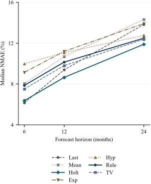
Last value had the lowest 6-month median NMAE (6.15%), versus Holt's 6.36% and the rule's 7.86%. Holt led at 12 and 24 months (8.64%, 11.89%; Table 3; Figure 1). Hyperbolic and mean errors rose from 9.98% to 12.76% and 8.05% to 14.32%. Rankings distinguish rapid level tracking from constrained extrapolation, but do not isolate duration from target calendar composition.

Download: Download full-size image

Figure 1. Model errors across forecast horizons.

At 24 months, median WAPE favored temporal selection (13.77%) over Holt (13.81%), reversing NMAE: WAPE uses future production, NMAE historical scale. Neither median production-weighted cases; all 659 WAPEs were defined (otherwise undefined WAPE alone would be excluded). The common set contained 656 cases/135 wells. Holt's NMAE medians were 6.17%, 8.48%, 11.88%, versus the rule's 7.56%, 10.00%, 12.47%, preserving the descriptive pattern at fixed composition.

3.2. Historical Trend Did Not Determine the Best Function

Table 4. Median 12-month NMAE by historical trend.

Method	Stable n=330	Declining n=166	Rising n=56	Insufficient n=119
Last value	8.06	11.29	5.91	10.25
Six-month mean	9.14	13.06	8.89	11.65
Holt damped	8.20	8.79	6.88	10.56
Exponential	9.86	12.30	16.33	11.41
Arps hyperbolic	10.14	12.58	18.30	9.60
Trend rule	9.14	12.58	6.88	11.65
Temporal selection	9.17	9.46	8.76	11.65

Values are percentages. Trend categories were determined from training data; every model used identical cases and scoring months within each category.

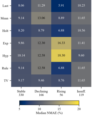
At 12 months, stable-history medians were 8.06% for last value, 8.20% for Holt, and 9.14% for the rule. In declining histories, Holt's 8.79% beat the assigned hyperbolic model's 12.58%. In rising histories, Holt's 6.88% beat exponential (16.33%) and hyperbolic (18.30%) but exceeded last value (5.91%). Insufficient-history hyperbolic error was 9.60%, versus the mean fallback's 11.65%. These retrospective subgroup comparisons do not validate replacement rules (Table 4; Figure 2).

Download: Download full-size image

Figure 2. Historical trend and model error.

At 24 months, declining-history medians were 19.96% (mean), 13.30% (hyperbolic), 12.98% (Holt), and 11.54% (temporal selection). Decline exposed constant-level limitations without uniquely identifying a reliable decline function. The rule sensibly avoided declining hyperbolic forecasts for rising histories, but its decline mapping restricted adaptation to later changes.

3.3. Selection Gains Depended on the Comparator and Uncertainty Model

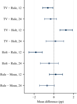
Temporal-selection medians were 7.51%, 9.80%, 12.38%, versus the rule's 7.86%, 10.14%, 12.49%. Its well-weighted paired differences from the rule were -0.61 pp at 12 months (95% interval -1.14 to -0.09) and -0.33 pp at 24 months (-0.94 to 0.27; Table 5; Figure 3). These are mean paired differences, not differences of case medians.

Table 5. Paired well-weighted NMAE differences and exploratory intervals.

Comparison	Horizon mo	Wells	Mean pp	95% interval pp
Rule - Mean	12	138	0.18	[-0.46, 0.89]
Rule - Mean	24	135	-0.69	[-1.46, 0.05]
TV - Rule	12	138	-0.61	[-1.14, -0.09]
TV - Rule	24	135	-0.33	[-0.94, 0.27]
Holt - Rule	12	138	-1.83	[-2.54, -1.17]
Holt - Rule	24	135	-0.48	[-1.37, 0.47]
TV - Holt	12	138	1.23	[0.62, 1.89]
TV - Holt	24	135	0.15	[-0.80, 1.01]
TV - Last	12	138	1.28	[0.57, 2.04]
TV - Last	24	135	-0.19	[-0.96, 0.58]

The first method minus the second is reported; negative values favor the first. pp, percentage points. Intervals are well-cluster bootstrap percentiles, conditional on the observed field and origins, without multiplicity adjustment.

Holt-minus-rule differences were -1.83 pp (-2.54 to -1.17) at 12 months and -0.48 pp (-1.37 to 0.47) at 24 months. Rule-minus-mean differences were 0.18 and -0.69 pp, both intervals crossing zero. Trend interpretability therefore did not provide a general predictive advantage.

Temporal selection exceeded Holt by 1.23 pp (0.62 to 1.89) and last value by 1.28 pp (0.57 to 2.04) at 12 months. Its 24-month difference from Holt was 0.15 pp (-0.80 to 1.01). Improvement over the rule did not establish improvement over strong baselines; these well-weighted means differ from Table 3's median rankings.

Leaving out individual origin years kept the 12-month temporal-minus-rule estimate within -0.75 to -0.44 pp. Crossed well/year resampling widened intervals to -1.47 to 0.11 at 12 months and -1.41 to 0.67 at 24 months, making the small gain sensitive to shared annual variation.

Download: Download full-size image

Figure 3. Paired forecast-error differences.

3.4. Future Trajectory Changes Exposed Extrapolation Limits

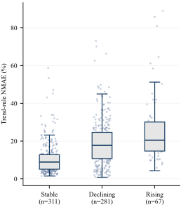
Retrospective 24-month groups contained 311 future-stable, 281 future-declining, and 67 future-rising cases, with rule medians of 8.94%, 17.74%, and 20.56% (Figure 4). Errors were larger when future levels departed from history. Because grouping and error share future observations, the association neither identifies causes nor predicts group membership in advance.

Download: Download full-size image

Figure 4. Errors grouped by retrospectively observed future trajectories.

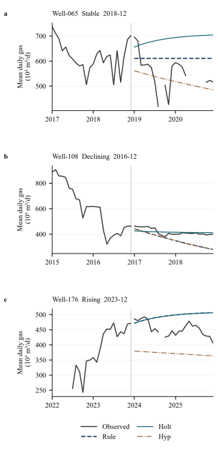
Illustrations used the median-position case after ordering each stable, declining, and rising historical group by 24-month rule NMAE. Well-065 (December 2018, level forecast) had 11.83% error; Well-108 (December 2016, hyperbolic) had 13.30%, with later observations nearer a plateau; Well-176 (December 2023, Holt) had 10.68% (Figure 5). The fixed rule avoids favorable-case selection and illustrates history–future differences. All codes are opaque replacements.

Download: Download full-size image

Figure 5. Illustrative trajectories selected by a fixed rule. Panels (a), (b), and (c) show median-position trend-rule-error cases within the stable, declining, and rising historical groups.

3.5. Validation Availability and Complete Index Correction

Requiring ≥20 days reduced horizon sets to 392, 387, and 371 cases. Holt's 12-/24-month medians were 7.91%/10.76%, below the rule's 10.11%/14.43%. The 12-month temporal-minus-rule mean attenuated to -0.10 pp (-0.51 to 0.27). Support changes altered history continuity, classification, and scoring samples together, preventing single-process attribution.

At 12 months, zero/one/two usable inner windows occurred in 171/125/375 primary cases versus 273/87/27 stricter-support cases. Identical selector outputs rose from 369/671 (55.0%) to 316/387 (81.7%). Among validation-eligible cases, temporal-minus-rule means were -0.81 pp for 119 wells (-1.73 to -0.02), versus -0.59 for 70 wells under stricter support (-1.93 to 0.57). Selection feasibility and sample composition both changed.

The 12-month support-set intersection contained 387 cases/134 wells. Temporal-minus-rule means were -0.32 pp at 10 days and -0.10 at 20 days, both intervals crossing zero. History length changed in 286 cases and category in 185; future scoring masks could also change. This compares complete pipelines on matching wells/origins, not one isolated factor.

Table 6. Median NMAE after index correction and candidate expansion.

Configuration	6 mo	12 mo	24 mo
Original hyperbolic	9.98	11.07	12.76
Aligned hyperbolic	9.77	10.74	12.51
Original trend rule	7.86	10.14	12.49
Aligned trend rule	7.56	10.14	12.40
Original TV, 4 models	7.51	9.80	12.38
Aligned TV, 4 models	7.47	9.81	12.38
Aligned TV, 5 models	7.16	9.29	12.09

Values are percentages. Aligned configurations start the hyperbolic forecast at t = n and apply the correction throughout internal validation and outer refitting. The five-model extension adds the last-value baseline and is exploratory.

Complete index correction yielded rule medians of 7.56%, 10.14%, 12.40% and four-model temporal medians of 7.47%, 9.81%, 12.38% (Table 6). Selections changed in 30/689 training cases. At 12 months, temporal-minus-rule was -0.58 pp (-1.11 to -0.08), but temporal selection exceeded Holt by 1.20 pp (0.62 to 1.86). The one-month discrepancy did not fully explain the rule's limitations.

Adding last value selected it in 152/689 training cases and reduced medians to 7.16%, 9.29%, 12.09%. The 12-month paired mean still exceeded Holt by 0.81 pp (0.24 to 1.45); the 24-month difference was -0.11 (-1.05 to 0.74). Candidate expansion improved locally without consistent superiority or independent deployment validation.

3.6. Origin-Year Heterogeneity and Local Threshold Sensitivity

Table 7. Median 12-month NMAE at each December origin.

Origin	Last	Mean	Holt	Rule	TV
2016-12	12.61	14.12	11.09	14.13	11.95
2017-12	8.76	9.69	9.85	11.65	10.93
2018-12	13.39	8.88	11.73	9.71	10.40
2019-12	9.11	8.71	9.57	8.37	8.71
2020-12	11.70	15.07	13.28	15.31	15.21
2021-12	8.99	10.71	6.52	9.20	9.81
2022-12	9.11	13.06	8.48	10.15	8.02
2023-12	5.84	9.02	5.93	6.58	6.54

Values are percentages. Each row uses its own eligible set; origin-year comparisons can reflect changing well composition. Model abbreviations are defined in Figure 1.

Holt did not lead at every origin (Table 7): last value beat it in December 2017 (8.76% versus 9.85%), and mean in December 2018 (8.88% versus 11.73%); Holt beat mean in December 2021 (6.52% versus 10.71%). Changing eligible wells prevents attribution to seasonality, allocation, or interventions. These are origin-year differences within the year-end design.

Training histories (n = 689) had median length 39 months (IQR 20–60). Stable, declining, and rising groups had medians of 48, 44, and 42.5 months and 24 months supporting earlier levels; insufficient histories had median length 15 months.

Table 8. Local sensitivity of the corrected trend rule.

Decline boundary	Rising boundary	History months	Changed labels	NMAE 12 mo	NMAE 24 mo
0.80	1.15	18	0	10.14	12.40
0.75	1.15	18	54	10.20	12.89
0.85	1.15	18	51	10.18	12.32
0.80	1.10	18	28	10.01	12.32
0.80	1.20	18	14	10.11	12.38
0.80	1.15	24	54	10.14	12.46

Values in the final two columns are percentages. Label changes are counted among 689 eligible training histories. One threshold was perturbed at a time, with scored cases held fixed; outer errors did not determine the perturbations.

Local threshold changes moved some histories between categories, while corrected-rule medians ranged 10.01%–10.20% at 12 months and 12.32%–12.89% at 24 months (Table 8). None beat Holt on identical cases. This concerns only the specified local configurations, not arbitrary thresholds or other fields.

4. Discussion

4.1. Daily Histories Define Conditional Extrapolation Performance

Production history and forecast scope require joint consideration. Last value follows current levels quickly; persistent decline undermines longer constant-level forecasts, while nonpersistent growth limits unrestricted extrapolation. Holt damping offered a favorable NMAE compromise here. This interpretation follows model structure and rankings, not controlled operating-condition experiments.

Unlike deep-sequence and physically constrained methods

[2, 3, 7, 9]

, this study documents simpler forecasts and their applicability. Bayesian decline models quantify probabilistic uncertainty

[4]

; multitask and pattern-matching methods share cross-well information

[6, 8]

. Their published errors cannot establish superiority here. Extensions require identical origins, targets, and metrics, with additional inputs and computational costs reported.

4.2. Interpretability and Predictive Gain Are Distinct Objectives

The rule's growth/trend, stability/level, and decline/hyperbolic mapping is interpretable, but a production ratio cannot distinguish allocation, pressure depletion, liquid loading, or interventions. Operational decline analysis

[5]

and hybrid forecasting

[10]

motivate richer observations and constraints. Wellhead pressure was not treated as bottomhole pressure, nor increasing water–gas ratio as proof of water invasion.

Temporal validation permits different functions within one trend class, but one or two windows cover limited conditions, and a 12-month criterion may poorly serve 24-month forecasts. Fallbacks make selectors identical in many cases. Gains depended on baselines, observation support, and annual resampling. Forecast combinations could reduce single-selection risk

[14]

, but were not tested.

4.3. Implications for Production Planning and Uncertainty

Well errors, field errors, and wrong trend directions answer different planning questions. Cancellation can hide well-level errors, and a large historical cumulative base can dilute relative error. Planning should assess future incremental volumes or consistently supported integration proxies before allocation constraints. New wells, interventions, and facility capacity were excluded, so existing-well extrapolation is not a complete field plan.

Application bands based on horizon and historical variability lack independent coverage validation and should not be labeled specified-confidence prediction intervals. Time-series conformal prediction offers an explicit coverage framework

[15]

, subject to nonstationarity and dependence. Our bootstrap intervals instead concern comparative error, not individual-well future production coverage.

4.4. Limitations and Testable Extensions

First, one field group may share geology, operations, allocation, and infrastructure; external performance remains unestablished. Contiguous-history and future-support eligibility underrepresents prolonged cessation and incomplete reporting. Observed-day means may be biased by selective omission of nonproduction days, which stricter support cannot resolve. Lifecycle evaluation requires verified cessation records and measurement definitions.

Second, parameters were finalized after evaluated origins, with possible development-backtest overlap despite past-only individual fits. Prospective testing after freezing functions and thresholds is needed. Eight origins and overlapping 24-month targets limit temporal replication even with crossed resampling; multi-origin assessment

[13]

cannot remove shared infrastructure effects or replace external validation. December-only origins confound duration with target calendar composition.

Third, four source functions and one baseline exclude uniformly tuned deep networks; the best tested function is not universally optimal. Verified intervention dates could test state-transition forecasts, pressure/water features incremental value, and rolling updates long-horizon deterioration. Each extension needs prediction-time inputs, nested temporal selection, and independent evaluation.

5. Conclusions

Across eight December origins, last value had the lowest pooled median NMAE at 6 months and Holt at 12 and 24 months, but rankings varied by year. These year-end existing-well results do not isolate a pure horizon effect.

Historical decline did not justify universal hyperbolic assignment, including after complete index correction. Temporal selection and last-value expansion improved locally over the rule without consistent gains over strong baselines. Validation availability and shared annual variation constrained gains; future-trajectory diagnoses remained retrospective.

Daily-report forecasting should document information availability, strong baselines, paired comparisons, and applicability. Interpretability, accuracy, and reservoir inference require distinct evidence. Findings support conditional analysis of adequately observed wells, pending prospective, external-field, and operationally informed validation.

Abbreviations

NMAE	Normalized Mean Absolute Error
WAPE	Weighted Absolute Percentage Error
sMAPE	Symmetric Mean Absolute Percentage Error
TV	Historical Temporal Validation Selection
pp	Percentage Points

Author Contributions

Zijie Wang: Conceptualization, Methodology, Writing – original draft

Haidong Shi: Funding acquisition, Project administration, Supervision, Writing – review & editing

Pengyu Chen: Data curation, Formal Analysis, Investigation

Degang Feng: Software, Validation, Visualization

Luming Cha: Resources, Validation

Siqi Wang: Investigation, Resources

Funding

This work is supported by CNODC R&D Project Topic "Research and Application of Efficient Development Technologies for Fractured-Porous Carbonate Gas Reservoirs" (2023ZZ19-05).

Conflicts of Interest

The authors declare that there are no conflicts of interest regarding the publication of this article.

References

[1]	Cao C., Jia P., Cheng L., Jin Q., Qi S. A review on application of data-driven models in hydrocarbon production forecast. Journal of Petroleum Science and Engineering, 2022, 212: 110296. https://doi.org/10.1016/j.petrol.2022.110296
[2]	Gu S., Wang J., Xue L., Tu B., Yang M., Liu Y. Deep-Learning-Based Production Decline Curve Analysis in the Gas Reservoir through Sequence Learning Models. Computer Modeling in Engineering & Sciences, 2022, 131(3): 1579-1599. https://doi.org/10.32604/cmes.2022.019435
[3]	Xue L., Wang J., Han J., Yang M., Mwasmwasa M. S., Nanguka F. Gas well performance prediction using deep learning jointly driven by decline curve analysis model and production data. Advances in Geo-Energy Research, 2023, 8(3): 159-169. https://doi.org/10.46690/ager.2023.06.03
[4]	Tadjer A., Hong A., Bratvold R. Bayesian Deep Decline Curve Analysis: A New Approach for Well Oil Production Modeling and Forecasting. SPE Reservoir Evaluation & Engineering, 2022, 25(3): 568-582. https://doi.org/10.2118/209616-PA
[5]	Jongkittinarukorn K., Last N. C., Kabir C. S. Decline-curve analysis with decline rate for improving reserves estimation in gas reservoirs. Gas Science and Engineering, 2023, 116: 205044. https://doi.org/10.1016/j.jgsce.2023.205044
[6]	Li X., Ma X., Xiao F., Xiao C., Wang F., Zhang S. Small-Sample Production Prediction of Fractured Wells Using Multitask Learning. SPE Journal, 2022, 27(3): 1504-1519. https://doi.org/10.2118/209231-PA
[7]	Gou L., Yang Z., Min C., Yi D., Li X., Kong B. A novel domain adaptation method with physical constraints for shale gas production forecasting. Applied Energy, 2024, 371: 123673. https://doi.org/10.1016/j.apenergy.2024.123673
[8]	Dong Y., Hao Y., Lu D. A framework for timely and accessible long-term forecasting of shale gas production based on time series pattern matching. International Journal of Forecasting, 2025, 41(2): 821-843. https://doi.org/10.1016/j.ijforecast.2024.07.009
[9]	Ma S., Zhang T., Wang H., Wang H., Li N., Zhu H., et al. Transformer-based forecasting for high-frequency natural gas production data. Energy and AI, 2025, 21: 100535. https://doi.org/10.1016/j.egyai.2025.100535
[10]	Raoof B. K., Rabia A., Alameedy U., Shakor P., Karakouzian M. Synergizing Machine Learning and Physical Models for Enhanced Gas Production Forecasting: A Comparative Study of Short- and Long-Term Feasibility. Energies, 2025, 18(5): 1187. https://doi.org/10.3390/en18051187
[11]	Petropoulos F., Apiletti D., Assimakopoulos V., Babai M. Z., Barrow D. K., Ben Taieb S., et al. Forecasting: theory and practice. International Journal of Forecasting, 2022, 38(3): 705-871. https://doi.org/10.1016/j.ijforecast.2021.11.001
[12]	Hewamalage H., Ackermann K., Bergmeir C. Forecast evaluation for data scientists: common pitfalls and best practices. Data Mining and Knowledge Discovery, 2023, 37(2): 788-832. https://doi.org/10.1007/s10618-022-00894-5
[13]	Ma S., Fildes R. The performance of the global bottom-up approach in the M5 accuracy competition: A robustness check. International Journal of Forecasting, 2022, 38(4): 1492-1499. https://doi.org/10.1016/j.ijforecast.2021.09.002
[14]	Wang X., Hyndman R. J., Li F., Kang Y. Forecast combinations: An over 50-year review. International Journal of Forecasting, 2023, 39(4): 1518-1547. https://doi.org/10.1016/j.ijforecast.2022.11.005
[15]	Xu C., Xie Y. Conformal Prediction for Time Series. IEEE Transactions on Pattern Analysis and Machine Intelligence, 2023, 45(10): 11575-11587. https://doi.org/10.1109/TPAMI.2023.3272339

Cite This Article

Plain Text BibTeX RIS

APA Style

Wang, Z., Shi, H., Chen, P., Feng, D., Cha, L., et al. (2026). Production Trend Stratification and Temporal Validation of Gas Well Forecasts from Daily Reports. International Journal of Energy and Environmental Science, 11(6), 141-151. https://doi.org/10.11648/j.ijees.20261106.11

Copy | Download

ACS Style

Wang, Z.; Shi, H.; Chen, P.; Feng, D.; Cha, L., et al. Production Trend Stratification and Temporal Validation of Gas Well Forecasts from Daily Reports. Int. J. Energy Environ. Sci. 2026, 11(6), 141-151. doi: 10.11648/j.ijees.20261106.11

Copy | Download

AMA Style

Wang Z, Shi H, Chen P, Feng D, Cha L, et al. Production Trend Stratification and Temporal Validation of Gas Well Forecasts from Daily Reports. Int J Energy Environ Sci. 2026;11(6):141-151. doi: 10.11648/j.ijees.20261106.11

Copy | Download

@article{10.11648/j.ijees.20261106.11,
  author = {Zijie Wang and Haidong Shi and Pengyu Chen and Degang Feng and Luming Cha and Siqi Wang},
  title = {Production Trend Stratification and Temporal Validation of Gas Well Forecasts from Daily Reports},
  journal = {International Journal of Energy and Environmental Science},
  volume = {11},
  number = {6},
  pages = {141-151},
  doi = {10.11648/j.ijees.20261106.11},
  url = {https://doi.org/10.11648/j.ijees.20261106.11},
  eprint = {https://article.sciencepublishinggroup.com/pdf/10.11648.j.ijees.20261106.11},
  abstract = {We tested whether historical production trends justify gas well forecast-model selection using 620,232 daily records from 178 pseudonymized wells. Fixed forecasts at eight December origins (2016-2023) were evaluated over 6, 12, and 24 months, retaining 678, 671, and 659 well–origin cases from 139, 138, and 135 wells. Comparators comprised level, damped-trend, and empirical decline functions, a fixed trend rule, and past-only temporal selection. The last-value baseline had the lowest median normalized mean absolute error (NMAE) at 6 months (6.15%); Holt's damped trend had the lowest at 12 and 24 months (8.64% and 11.89%), versus 10.14% and 12.49% for the trend rule. At 12 months, temporal selection reduced well-weighted mean NMAE by 0.61 percentage points relative to the rule (well-cluster bootstrap 95% interval: -1.14 to -0.09), but the interval crossed zero when origin years were also resampled. Temporal selection still exceeded Holt's error by 1.23 percentage points. Consistently correcting hyperbolic forecast indexing in inner validation and outer prediction preserved the main conclusions. Historical decline did not uniquely identify the most reliable function, and added selection steps did not consistently improve on strong simple baselines. These findings apply to adequately observed existing wells at year-end origins and require prospective and external-field validation.},
 year = {2026}
}

Copy | Download

TY  - JOUR
T1  - Production Trend Stratification and Temporal Validation of Gas Well Forecasts from Daily Reports
AU  - Zijie Wang
AU  - Haidong Shi
AU  - Pengyu Chen
AU  - Degang Feng
AU  - Luming Cha
AU  - Siqi Wang
Y1  - 2026/11/10
PY  - 2026
N1  - https://doi.org/10.11648/j.ijees.20261106.11
DO  - 10.11648/j.ijees.20261106.11
T2  - International Journal of Energy and Environmental Science
JF  - International Journal of Energy and Environmental Science
JO  - International Journal of Energy and Environmental Science
SP  - 141
EP  - 151
PB  - Science Publishing Group
SN  - 2578-9546
UR  - https://doi.org/10.11648/j.ijees.20261106.11
AB  - We tested whether historical production trends justify gas well forecast-model selection using 620,232 daily records from 178 pseudonymized wells. Fixed forecasts at eight December origins (2016-2023) were evaluated over 6, 12, and 24 months, retaining 678, 671, and 659 well–origin cases from 139, 138, and 135 wells. Comparators comprised level, damped-trend, and empirical decline functions, a fixed trend rule, and past-only temporal selection. The last-value baseline had the lowest median normalized mean absolute error (NMAE) at 6 months (6.15%); Holt's damped trend had the lowest at 12 and 24 months (8.64% and 11.89%), versus 10.14% and 12.49% for the trend rule. At 12 months, temporal selection reduced well-weighted mean NMAE by 0.61 percentage points relative to the rule (well-cluster bootstrap 95% interval: -1.14 to -0.09), but the interval crossed zero when origin years were also resampled. Temporal selection still exceeded Holt's error by 1.23 percentage points. Consistently correcting hyperbolic forecast indexing in inner validation and outer prediction preserved the main conclusions. Historical decline did not uniquely identify the most reliable function, and added selection steps did not consistently improve on strong simple baselines. These findings apply to adequately observed existing wells at year-end origins and require prospective and external-field validation.
VL  - 11
IS  - 6
ER  -

Copy | Download

Author Information

Zijie Wang

CNPC Science and Technology Research Institute, Beijing, China
Haidong Shi

CNPC Science and Technology Research Institute, Beijing, China

Contact Email
Pengyu Chen

CNPC Science and Technology Research Institute, Beijing, China
Degang Feng

China National Oil and Gas Exploration and Development Company Ltd, Beijing, China
Luming Cha

CNPC Science and Technology Research Institute, Beijing, China
Siqi Wang

CNPC Science and Technology Research Institute, Beijing, China

Download PDF

Submit an Article

Plain Text BibTeX RIS

APA Style

Wang, Z., Shi, H., Chen, P., Feng, D., Cha, L., et al. (2026). Production Trend Stratification and Temporal Validation of Gas Well Forecasts from Daily Reports. International Journal of Energy and Environmental Science, 11(6), 141-151. https://doi.org/10.11648/j.ijees.20261106.11

Copy | Download

ACS Style

Wang, Z.; Shi, H.; Chen, P.; Feng, D.; Cha, L., et al. Production Trend Stratification and Temporal Validation of Gas Well Forecasts from Daily Reports. Int. J. Energy Environ. Sci. 2026, 11(6), 141-151. doi: 10.11648/j.ijees.20261106.11

Copy | Download

AMA Style

Wang Z, Shi H, Chen P, Feng D, Cha L, et al. Production Trend Stratification and Temporal Validation of Gas Well Forecasts from Daily Reports. Int J Energy Environ Sci. 2026;11(6):141-151. doi: 10.11648/j.ijees.20261106.11

Copy | Download

@article{10.11648/j.ijees.20261106.11,
  author = {Zijie Wang and Haidong Shi and Pengyu Chen and Degang Feng and Luming Cha and Siqi Wang},
  title = {Production Trend Stratification and Temporal Validation of Gas Well Forecasts from Daily Reports},
  journal = {International Journal of Energy and Environmental Science},
  volume = {11},
  number = {6},
  pages = {141-151},
  doi = {10.11648/j.ijees.20261106.11},
  url = {https://doi.org/10.11648/j.ijees.20261106.11},
  eprint = {https://article.sciencepublishinggroup.com/pdf/10.11648.j.ijees.20261106.11},
  abstract = {We tested whether historical production trends justify gas well forecast-model selection using 620,232 daily records from 178 pseudonymized wells. Fixed forecasts at eight December origins (2016-2023) were evaluated over 6, 12, and 24 months, retaining 678, 671, and 659 well–origin cases from 139, 138, and 135 wells. Comparators comprised level, damped-trend, and empirical decline functions, a fixed trend rule, and past-only temporal selection. The last-value baseline had the lowest median normalized mean absolute error (NMAE) at 6 months (6.15%); Holt's damped trend had the lowest at 12 and 24 months (8.64% and 11.89%), versus 10.14% and 12.49% for the trend rule. At 12 months, temporal selection reduced well-weighted mean NMAE by 0.61 percentage points relative to the rule (well-cluster bootstrap 95% interval: -1.14 to -0.09), but the interval crossed zero when origin years were also resampled. Temporal selection still exceeded Holt's error by 1.23 percentage points. Consistently correcting hyperbolic forecast indexing in inner validation and outer prediction preserved the main conclusions. Historical decline did not uniquely identify the most reliable function, and added selection steps did not consistently improve on strong simple baselines. These findings apply to adequately observed existing wells at year-end origins and require prospective and external-field validation.},
 year = {2026}
}

Copy | Download

TY  - JOUR
T1  - Production Trend Stratification and Temporal Validation of Gas Well Forecasts from Daily Reports
AU  - Zijie Wang
AU  - Haidong Shi
AU  - Pengyu Chen
AU  - Degang Feng
AU  - Luming Cha
AU  - Siqi Wang
Y1  - 2026/11/10
PY  - 2026
N1  - https://doi.org/10.11648/j.ijees.20261106.11
DO  - 10.11648/j.ijees.20261106.11
T2  - International Journal of Energy and Environmental Science
JF  - International Journal of Energy and Environmental Science
JO  - International Journal of Energy and Environmental Science
SP  - 141
EP  - 151
PB  - Science Publishing Group
SN  - 2578-9546
UR  - https://doi.org/10.11648/j.ijees.20261106.11
AB  - We tested whether historical production trends justify gas well forecast-model selection using 620,232 daily records from 178 pseudonymized wells. Fixed forecasts at eight December origins (2016-2023) were evaluated over 6, 12, and 24 months, retaining 678, 671, and 659 well–origin cases from 139, 138, and 135 wells. Comparators comprised level, damped-trend, and empirical decline functions, a fixed trend rule, and past-only temporal selection. The last-value baseline had the lowest median normalized mean absolute error (NMAE) at 6 months (6.15%); Holt's damped trend had the lowest at 12 and 24 months (8.64% and 11.89%), versus 10.14% and 12.49% for the trend rule. At 12 months, temporal selection reduced well-weighted mean NMAE by 0.61 percentage points relative to the rule (well-cluster bootstrap 95% interval: -1.14 to -0.09), but the interval crossed zero when origin years were also resampled. Temporal selection still exceeded Holt's error by 1.23 percentage points. Consistently correcting hyperbolic forecast indexing in inner validation and outer prediction preserved the main conclusions. Historical decline did not uniquely identify the most reliable function, and added selection steps did not consistently improve on strong simple baselines. These findings apply to adequately observed existing wells at year-end origins and require prospective and external-field validation.
VL  - 11
IS  - 6
ER  -

Copy | Download